Appendix P — Quiz 2

P.1 A. Single Choice Questions (4%, 48%)

P.1.1 (1) Which of the following statements is False?

1. The super() function is a specific function that enables calling a method from the parent class.

2. The cls parameter functions similarly to self, but instead of referring to an object, it refers to the class of an object.

3. In the Python class, the self parameter is required in the definition of every method, and it must come first before any other parameters.

4. If we directly access an attribute starting with __, an error will occur.

Ans: (C) In Python, the self parameter is not required in the definition of every method. Specifically, it is not used in @staticmethods or @classmethods.

P.1.2 (2) When we directly evaluate (like when you type the object’s name and hit shift+enter) an object in the Jupyter Notebook, which special method will be called first?

1. __del__

2. __repr__

3. __str__

4. __init__

Ans: (B)

P.1.3 (3) Which of the following statements is False?

1. The Float class in SymPy can be used to represent a floating-point number, but the precision of the results is limited.

2. Using the evalf() method in SymPy makes it possible to evaluate an expression and obtain the result as a floating-point number.

3. SymPy is distinct from numerical libraries because it is created to perform algebraic manipulations symbolically, which allows us to obtain exact solutions to mathematical problems.

4. In SymPy, certain operations are not executed instantaneously. Instead, they generate an unevaluated object, which can be later evaluated by invoking the doit() method.

Ans: (A) The Float class in SymPy indeed allows us to represent floating-point numbers, but unlike standard floating-point numbers in Python (which have a fixed precision), the precision of a Float in SymPy can be arbitrarily high!

P.1.4 (4) By default, what will be printed out when we execute the following code snippet?

import sympy as sp
x,y = sp.symbols('x,y') # you can create multiple symbols at once using multiple assignment
(x + 2)*(x + 1)

1. \((x+1)(x+2)\)

2. \(x^2+3x+2\)

3. \(1+2x+x^2\)

4. \((x+2)(x+1)\)

Ans: (A)

P.1.5 (5) Which of the following statements is True?

1. The main difference between the array methods reshape() and resize() is that the resize() returns a view of the original array while reshape() returns a deep copy of the original array.

2. The main difference between the array methods ravel() and flatten() is that the ravel() returns a view of the original array while flatten() returns a deep copy of the original array.

3. In NumPy, the speed of for loop will usually be faster than vectorized operation when performing the element-wise operation.

4. In NumPy, to perform an element-wise operation between two arrays, the two arrays must have the same shape.

Ans: (B).

1. the reshape() function returns a new array that has the same data but a different shape, and it usually returns a view, not a deep copy. The resize() function changes the shape and size of array in-place.

2. vectorized operations are usually much faster than for loops due to the fact that vectorized operations take advantage of low-level optimizations and parallelism, which are not available when manually looping over the elements of the array.

3. For element-wise operations between two arrays in NumPy, they do not need to be the exact same shape due to broadcasting rules. Broadcasting allows operations to be performed on arrays of different sizes and/or dimensions, given certain conditions are met.

P.1.6 (6) Which of the following statement is False?

1. The array attribute size is the product of the shape tuple’s values. For instance, an array with three rows of two elements each will have a size equal to 6.

2. When we call the linspace() function to create an array, the endpoint will be included in the array by default.

3. The main difference between the built-in function random.randint() and the np.random.randint() is that the former will exclude the endpoint while the latter will not.

4. When we use the reduction function on a 2D array and specify axis=0, the calculation will be performed on all the row values within each column.

Ans: (C) The main difference between the built in function random.randint() and the np.random.randint() is that the former will include the endpoint while the latter will not.

P.1.7 (7) Which of the following is not a correct function/method mapping between the functional interface and the OOP interface in matplotlib?

1. plt.xlabel() -> ax.set_xlabel()

2. plt.ylim() -> ax.set_ylim()

3. plt.legend() -> ax.set_legend()

4. plt.title() -> ax.set_title()

Ans: (C)

P.1.8 (8) Which of the following statement is True?

1. To define a new class in Python we always need to implement the constructor __init__ and the destructor __del__ method.

2. The inheritance describes the “has a” relationship between two classes.

3. A static method is a special method that can access the attributes or methods of the class (using cls) or its objects (using self).

4. Operator overloading, which enables operators to exhibit varying behavior depending on the object types they interact with, is also an aspect of polymorphism.

Ans: (D). (A) Usually, we do not have to define __del__. (B) Should be composition. (C) static method can not access these two kinds of method or attribute.

P.1.9 (9) In the command plt.plot(x, y, '-bo'), what does the format string '-bo' mean?

1. Draw a solid line with black color and circle marker.

2. Draw a dotted line with black color and circle marker.

3. Draw a dotted line with blue color and square marker.

4. Draw a solid line with blue color and circle marker.

Ans: (D)

P.1.10 (10) Which of the following statements is False?

1. In SymPy, the terms of an expression are arranged according to the powers of x, in descending order, starting from the highest power to the lowest.

2. SymPy will not perform any simplification or expansion for an expression unless explicitly requested to do so.

3. Both solve() and nroots() can be used to find the roots of an equation, but the former will return the roots as numerical values while the latter will return the roots as symbolic expressions.

4. The high-order term O(x^n) after the series expansion can be eliminated by using the removeO() method.

Ans: (C) nroots() does not return the roots as symbolic expressions, but as numerical approximations.

P.1.11 (11) Which of the following statement is False?

1. The plt.text() function allows us to position text at a specific x/y coordinate, while the plt.annotate() function provides the ability to create text along with an arrow.

2. In the plt.scatter() function, we can use the alpha keyword to adjust the transparency level of each data point.

3. Although a significant number of plt functions (functional interface) have corresponding ax methods (OOP interface) with identical names, this rule does not hold universally for all commands.

4. Spines represent the lines that link the tick marks on the axes and delineate the data area. Typically, they are located at the center of the figure by default.

Ans: (D) They are at the border of the figure by default.

P.1.12 (12) If we would like to calculate c = a + b, which of the following arrays a and b will satisfy the broadcasting rules?

1. a = np.array([1, 2, 3]); b = np.array([4, 5, 6, 7])

2. a = np.array([[1, 2, 3], [4, 5, 6]]); b = np.array([[1, 2], [3, 4]])

3. a = np.array([[1, 2, 3], [4, 5, 6]]); b = np.array([7, 8])

4. a = np.array([[1, 2, 3]]); b = np.array([[1], [2]])

Ans: (D)

1. When the number of dimensions between two arrays differs, the array with fewer dimensions is padded with ones on its leading (left) side to match the number of dimensions of the other array.
2. If the shape of the two arrays doesn’t match in any dimension, the array with a shape of 1 in that dimension is expanded to match the shape of the other array.
3. If the sizes of the arrays conflict in any dimension and neither is equal to 1, an error is raised.

P.2 B. Short-answer and coding questions

import matplotlib as mpl
import matplotlib.pyplot as plt
import numpy as np
import sympy as sp
plt.style.use('seaborn-whitegrid')

C:\Users\adm\AppData\Local\Temp\ipykernel_29012\3720340587.py:5: MatplotlibDeprecationWarning: The seaborn styles shipped by Matplotlib are deprecated since 3.6, as they no longer correspond to the styles shipped by seaborn. However, they will remain available as 'seaborn-v0_8-<style>'. Alternatively, directly use the seaborn API instead.
  plt.style.use('seaborn-whitegrid')

P.2.1 (13) Considering the following Fraction class that has two attributes, num and den try to complete the following tasks: (8%)

1. Create a dunder method for the class so that two objects from the class can be added together.
2. When the user prints out the Fraction object, show the object in the form of a rational number and floating number.
3. Inherit the Fraction class and create a new class called integer that can be added to the Fraction class and when printing out the integer object, do not show the denominator part.

class Fraction():
    def __init__(self, numerator, denominator):
        self.set_num_den(numerator, denominator)

    def set_num_den(self, numerator, denominator):
        self.__num = numerator
        self.__den = denominator

    def get_num_den(self):
        return self.__num, self.__den
    
    # dunder method
    def __add__(self, otherfrac):
        newnum = self.__num * otherfrac.__den + self.__den* otherfrac.__num
        newden = self.__den * otherfrac.__den
        return Fraction(newnum, newden)
    
    def __str__(self):
        return f"{self.__num}/{self.__den}, {self.__num/self.__den}"
    
class integer(Fraction):
    def __init__(self, numerator):
        super().__init__(numerator, 1)
        
    def __str__(self):
        num, den = super().get_num_den() #getter
        return f"{num}"

# Test the class
x = Fraction(1,3)
y = integer(2)
print(y)
z = x + y
print(z)
print(z.get_num_den())

2
7/3, 2.3333333333333335
(7, 3)

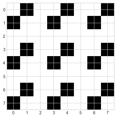
P.2.2 (14) Suppose we are developing a chess game and the chess game provides a special checkerboard as follows: (8%)

# The checkerboard

We decide to use 1 to represent the white square and 0 to represent the black square. Write a program to create two 2D arrays to represent the checkerboards. Note you should not directly hardcode the above arrays. You should use NumPy methods to create the arrays. After you have finished the exercise, you can print out the checkerboard using the following code cell. Finally, calculate the number of pixels of the back area and the white area, respectively, using NumPy.

checkerboard = np.ones((8, 8))
checkerboard[::3, 1::3] = 0
checkerboard[1::3, ::3] = 0
checkerboard

array([[1., 0., 1., 1., 0., 1., 1., 0.],
       [0., 1., 1., 0., 1., 1., 0., 1.],
       [1., 1., 1., 1., 1., 1., 1., 1.],
       [1., 0., 1., 1., 0., 1., 1., 0.],
       [0., 1., 1., 0., 1., 1., 0., 1.],
       [1., 1., 1., 1., 1., 1., 1., 1.],
       [1., 0., 1., 1., 0., 1., 1., 0.],
       [0., 1., 1., 0., 1., 1., 0., 1.]])

plt.imshow(checkerboard, cmap='gray');

white_area = np.sum(checkerboard)
black_area = 8*8 - np.sum(checkerboard)
int(white_area), int(black_area)

(46, 18)

Ans: The white area contains 46 pixels while the black area occupies 18 pixels.

P.2.3 (15) The definite integral represents the area under the curve of the graph of \(y=f(x)\) on the interval \([a,b]\). (10%)

\[ \int_a^b f(x) \, dx = \text{area under the curve } y = f(x) \text{ on } [a,b] \]

Note that the area above the \(x\)-axis is considered positive, while the area below the \(x\)-axis counts as negative area. Try to visualize the integral:

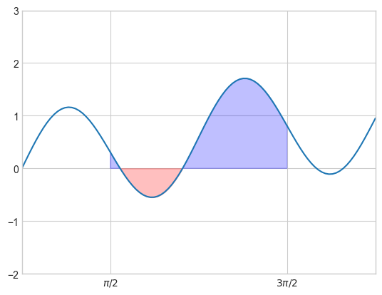
\[ \int_{\pi/2}^{3\pi/2} \left( \sin(0.2 x) + \sin(2x)\right) dx \] (8%).

You need to draw the curve of \(y = \sin(0.2 x) + \sin(2x)\) and use blue and red color to fill the positive and negative area respectively. Finally, calculate the area of the integral from \(\pi/2\) to \(3\pi/2\) using SymPy. Your result should be a floating number.

def f(x):
    return np.sin(0.2*x) + np.sin(2*x)

x = np.linspace(0,2*np.pi,100)
y = f(x)
plt.plot(x,y)

X = np.linspace(np.pi/2,3*np.pi/2,100)
Y = f(X)
plt.fill_between(X, 0, Y, Y > 0, color='blue', alpha=.25)
plt.fill_between(X, 0, Y, Y < 0, color='red',  alpha=.25)

plt.xticks([np.pi/2,3*np.pi/2],['$\pi/2$','$3\pi/2$'])
plt.xlim([0,2*np.pi]); plt.ylim([-2,3]);

x = sp.Symbol('x')
f = sp.sin(0.2*x) + sp.sin(2*x)
# sp.Integral(sp.sin(x), (x, 0, sp.pi / 2)).doit()
sp.integrate(f, (x, sp.pi/2, sp.pi*3/2)).evalf()

\(\displaystyle 1.8163563200134\)

P.2.4 (16) In this problem, we will compare two approaches to approximate the \(\arctan(1)\) using the sum of infinite series. (8%)

1. Fisrtly, write a program that computes the value of \(\pi\) from the following infinite series \(\arctan(x) = \sum_0^{\infty}(-1)^n\frac{x^{2n+1}}{(2n+1)}\) using NumPy by substitute x=1.
2. Secondly, expand the \(\arctan(x)\) using Taylor serise at \(x=0\) using SymPy.
3. Finally, set the number of terms for both approximations to 100 and make sure they agree with each other. (8%)

Hint: You may find lambdify() useful to convert a symbolic expression to a function that can be evaluated numerically.

n = 100
k = np.arange(0, n)
t1 = np.sum((-1)**(k) / (2*k + 1))

taylor = sp.series(sp.atan(x), x, 0, 200).removeO()
evaltaylor = sp.utilities.lambdify(x, taylor, modules=['numpy'])
t2 = evaltaylor(1)

np.isclose(t1, t2)

True

P.2.5 (17) In this problem, we will compare two approaches to calculate the roots of a given function \(x^3+3x^2+x-1\). (10%)

1. First, generate evenly spaced numbers between \(-3\) and \(3\).
2. Secondly, explain the functionality of sign(), diff() and nonzero() in NumPy.
3. Thirdly, use the above function to find where the function crosses the x-axis (the roots of the function) by substitution.
4. Finally, use SymPy to find the roots of the function (set the number of digits of the decimal part to 3) and make sure that they agree with each other.

Hint: You may need to adjust the number of evenly spaced points in the first step to get the same result.

• np.sign(): This function returns an element-wise indication of the sign of a number. It returns -1 for negative numbers, 0 for zero, and 1 for positive numbers.

• np.diff(): This function calculates the n-th discrete difference along the given axis. The first difference is given by out[n] = a[n+1] - a[n] along the given axis.

• np.nonzero(): This function returns the indices of the elements that are non-zero.

N = 2000
x = np.linspace(-3, 3, N)
y = x**3 + 3*x**2+ x -1
idx = np.nonzero(np.diff(np.sign(y)))
roots1 = x[idx]
roots1

array([-2.41437072, -1.00010001,  0.41417071])

x = sp.Symbol('x')
expr = x**3 + 3*x**2+ x -1
roots2 = sp.nroots(expr, n=3)
roots2

[-2.41, -1.00, 0.414]

np.isclose(roots1, np.array(roots2, dtype=np.float32), atol=1e-2)

array([ True,  True,  True])

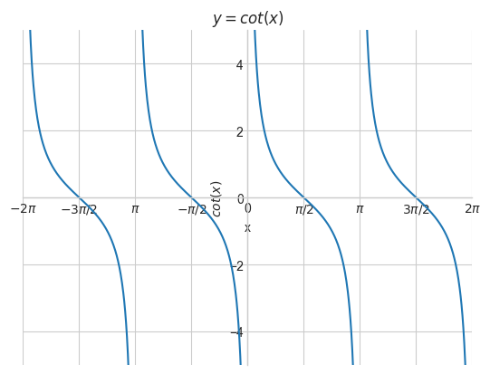
P.2.6 (18) Try to plot \(cot(x)\) using plot() function and set the limit of x between \([-2\pi, 2\pi]\). In addition, you need to move the spline to the center, add the title and change the ticks of the figure so that the plot looks as follows: (8%)

# The plot
def cotan(x):
    return np.cos(x)/np.sin(x)

x = np.linspace(-2 * np.pi, 2 * np.pi, 1000)
y = cotan(x)

y[np.isclose(x, np.pi, rtol=1e-02)] = np.nan
y[np.isclose(x, 0, atol=1e-02)] = np.nan
y[np.isclose(x, -np.pi, rtol=1e-02)] = np.nan

plt.xlabel("x")
plt.ylabel("$cot(x)$")
plt.xlim(-2 * np.pi, 2 * np.pi)
plt.ylim(-5, 5)
plt.title("$y = cot(x)$")
plt.plot(x, y)

radian_multiples = [-2, -3/2, -1, -1/2, 0, 1/2, 1, 3/2, 2]
radians = [n * np.pi for n in radian_multiples]
radian_labels = ['$-2\pi$', '$-3\pi/2$', '$\pi$', '$-\pi/2$', '0', '$\pi/2$', '$\pi$', '$3\pi/2$', '$2\pi$']

plt.xticks(radians, radian_labels);

ax = plt.gca()
ax.spines[['top', 'right']].set_visible(False)
ax.spines['bottom'].set_position(('data',0))
ax.spines['left'].set_position(('data',0))