package_name = "sympy"

try:
    __import__(package_name)
    print(f"{package_name} is already installed.")
except ImportError:
    print(f"{package_name} not found. Installing...")
    %pip install {package_name}
sympy is already installed.SymPy|
|

|
SymPy is a Python library designed for symbolic mathematics. Its goal is to serve as an alternative to systems like Mathematica, Maple, or Sage while maintaining a simple and easily extensible codebase. SymPy is written entirely in Python and does not necessitate any external libraries.
The standard way of importing the module is:
package_name = "sympy"
try:
__import__(package_name)
print(f"{package_name} is already installed.")
except ImportError:
print(f"{package_name} not found. Installing...")
%pip install {package_name}sympy is already installed.When you call sp.init_printing(), it sets up your session to be able to print SymPy objects in a more visually appealing and understandable way.
SymPy as a calculatorThe core module in the SymPy package includes the Number class, which represents atomic numbers. This class has two subclasses: the Float and Rational classes. The Rational class is further extended by the Integer class. First, let’s create an Integer object from SymPy and perform some calculations:
As demonstrated, if an exact result can be obtained, SymPy will return it. If not, SymPy will provide an expression instead.
The Rational class represents a rational number as a pair of two Integers: the numerator and the denominator. Thus, Rational(1, 2) represents 1/2, Rational(5, 2) represents 5/2, and so on:
Lastly, there is a Float class that can represent a floating-point number with arbitrary precision:
Note that this is in contrast to normal Python where we may get approximated results:
For more about the discussion of floating point math, see here or here for more information.
In addition to the numerical classes, SymPy features constant objects, such as pi, E, oo (infinity) and others. SymPy employs mpmath in the background, enabling computations using arbitrary-precision arithmetic. Consequently, certain special constants, like \(e\), \(\pi\), and \(\infty\), can also be evaluated:
As demonstrated, the evalf() method can be used to evaluate an expression as a floating-point number. To evaluate results with arbitrary precision, simply pass the desired number of digits to the evalf() method:
\(\displaystyle 1.414213562373095048801688724209698078569671875376948073176679737990732478462107038850387534327641573\)
As we have mentioned, there is also a object representing mathematical infinity called oo:
Finally, we also have other common functions like sin, cos, tan, exp, log, etc. in SymPy:
Symbols serve as the foundation of symbolic math. When we write the statement \(x + x + 1\), Python evaluates it, resulting in a numerical value. But what if we want the result in terms of the symbol \(x\)? SymPy enables us to write programs where we can express and evaluate mathematical expressions using such symbols. First, we import the Symbol class from SymPy and create an object of this class, passing 'x' as a parameter:
\(\displaystyle 2 x + 1\)
After defining symbols, you can perform basic mathematical operations on them using the same operators you’re already familiar with:
x,y = sp.symbols('x,y') # you can create multiple symbols at once using multiple assignment
p = (x + 3)*(y/3+x)
p
\(\displaystyle \left(x + 3\right) \left(x + \frac{y}{3}\right)\)
Note that symbols() is a function while Symbol is a class!
You might have anticipated that SymPy would multiply everything out. However, SymPy only automatically simplifies the most elementary expressions and requires the programmer to explicitly request further simplification. To expand an expression, utilize the expand() function:
You can also factor expressions using the factor() function:
The terms are organized in the order of x powers, from highest to lowest. If you prefer the expression in the reverse order, with the highest power of x appearing last, you can achieve that using the init_printing() function, as shown below:
The above code demonstrates that we want SymPy to display the expressions in reverse lexicographical order. In this instance, the keyword argument instructs Python to print terms with lower powers first.
We can also employ SymPy to substitute values into an expression. This allows us to compute the value of the expression for specific variable values. Take the mathematical expression \(x^2 + 2xy + y^2\), which can be defined as follows:
To evaluate this expression, you can substitute numbers for the symbols by using the subs() method:
Additionally, you can express one symbol in terms of another and perform substitutions accordingly, using the subs() method. For instance, if you know that \(x = 1 - y\), this is how you could evaluate the previous expression:
If you desire a more simplified result — for example, if there are terms that cancel each other out — you can utilize SymPy’s simplify() function:
sp.simplify(p3.subs({x:1-y})) # The result turns out to be 1 because the other terms of the expression cancel each other.\(\displaystyle 1\)
This example reiterates that SymPy will not perform any complex simplification unless explicitly requested to do so.
11.3.1 Exercise 1: Try to solve the following problems using
SymPy:Expand the following expression: \(\sin(4x)\cos(5x)\) so that the final results only contains
sin(x)and its power term (\(\sin^n(x)\)).
Hint: You can use simplify(), subs() and expand() function to simplify the expression. You may find keyowrd trig=True argument in expand() function useful. Finally, if you want to perform symbolic manipulation, be sure to use functions in SymPy.
SymPy’s solve() function can be employed to find solutions to equations. When you input an expression with a symbol representing a variable, such as x, solve() computes the value of that symbol. This function always performs its calculation by assuming the expression you enter is equal to zero — that is, it outputs the value that, when substituted for the symbol, makes the entire expression equal zero.
Let’s start with the simple equation \(x - 5 = 7\). If we want to use solve() to find the value of x, we first need to make one side of the equation equal zero (\(x - 5 - 7 = 0\)). Then, we’re ready to use solve(), as shown below:
Observe that the result 12 is returned within a list. An equation can have multiple solutions — for instance, a quadratic equation has two solutions. In such cases, the list will include all the solutions as its elements. Let’s look at an example:
\(\displaystyle \left( \left[ -4, \ -1\right], \ \left[ \left\{ x : -4\right\}, \ \left\{ x : -1\right\}\right]\right)\)
It’s worth noting that we can set dict=True as an argument to retrieve a dictionary instead of a list.
In addition to finding the roots of equations, we can leverage symbolic math to utilize the solve() function to express one variable in an equation in terms of the others. Let’s examine finding the roots for the general quadratic equation \(ax^2 + bx + c = 0\). To accomplish this, we’ll define x and three additional symbols — a, b, and c, which correspond to the three coefficients:
x = sp.Symbol('x')
a = sp.Symbol('a')
b = sp.Symbol('b')
c = sp.Symbol('c')

expr = a*x*x + b*x + c
sp.solve(expr, x, dict=True)
\(\displaystyle \left[ \left\{ x : \frac{- b - \sqrt{- 4 a c + b^{2}}}{2 a}\right\}, \ \left\{ x : \frac{- b + \sqrt{- 4 a c + b^{2}}}{2 a}\right\}\right]\)
In this example, we must include an additional argument, x, to the solve() function. Because there’s more than one symbol in the equation, we need to inform solve() which symbol it should solve for, which we indicate by passing in x as the second argument. As anticipated, solve() outputs the quadratic formula: the general formula for determining the value(s) of x in a polynomial expression.
We can also sove the expression using nsolve() function. nsolve() function is a numerical solver that uses numerical methods to find the roots of an equation given a starting point. For example, we can solve the equation \(x^2 - 2 = 0\) using nsolve() function:
x = sp.Symbol('x')
expr = x**2 - 2
sp.nsolve(expr, -1), sp.nsolve(expr, 1), sp.solve(expr) # -1 and 1 are the starting points
\(\displaystyle \left( -1.4142135623731, \ 1.4142135623731, \ \left[ - \sqrt{2}, \ \sqrt{2}\right]\right)\)
Consider the following two equations:
\[ \begin{align} 2x + 3y &= 6 \\ 3x + 2y &= 12 \end{align} \]
Suppose we want to find the pair of values (x, y) that satisfies both equations. We can use the solve() function to find the solution for a system of equations like this one. First, we define the two symbols and construct the two equations:
x = sp.Symbol('x')
y = sp.Symbol('y')
expr1 = 2*x + 3*y - 6
expr2 = 3*x + 2*y - 12

sp.solve((expr1, expr2), dict=True) # Enclose the equations in a tuple
\(\displaystyle \left[ \left\{ x : \frac{24}{5}, \ y : - \frac{6}{5}\right\}\right]\)
Observe how we’ve rearranged the expressions so that they both equal zero. Retrieving the solution as a dictionary is beneficial in this scenario because we can verify whether the solution we obtained indeed satisfies the equations:
sol = sp.solve((expr1, expr2), dict=True)
expr1.subs({x:sol[0][x], y:sol[0][y]}), expr2.subs({x:sol[0][x], y:sol[0][y]})
\(\displaystyle \left( 0, \ 0\right)\)
The output of substituting the values of x and y corresponding to the solution in the two expressions is zero, which confirms that the solution satisfies both equations.
If we’re unable to obtain the exact solution, we can still obtain the numerical solution using the nroots() function:
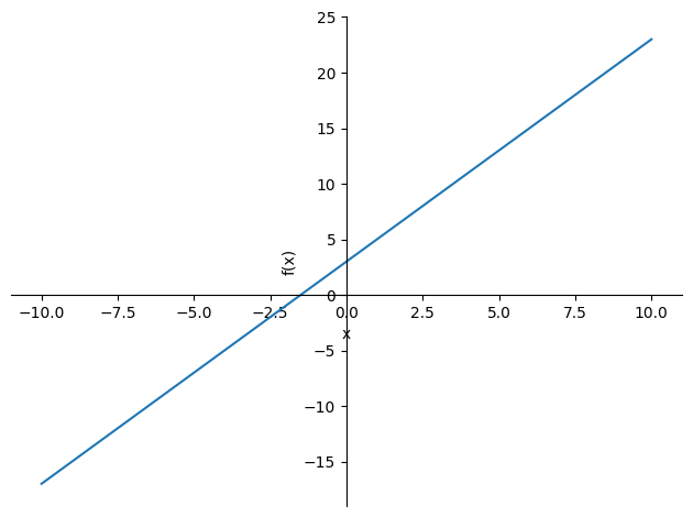
SymPyWith SymPy, you can simply provide the equation of the line you wish to plot, and SymPy will create the graph for you. Let’s plot a line whose equation is given by \(y = 2x + 3\):
The graph reveals that a default range of
xvalues was automatically selected: −10 to 10. In reality,SymPyemploysmatplotlibin the background to generate the graphs.
Suppose you wanted to constrain the values of x in the previous graph to lie within the range of −5 to 5. Additionally, we can use other keyword arguments in the plot() function, such as title to specify a title or xlabel and ylabel to label the x-axis and the y-axis, respectively. Here’s how to accomplish this:
sp.plot(2*x + 3, (x, -5, 5), title='A Line', xlabel='x', ylabel='2x+3'); #(symbol, start, end) to specify the range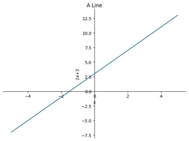
You can plot more than one expression on the same graph by providing multiple expressions when calling the SymPy plot() function. Here’s the code:
x = sp.Symbol('x')
p = sp.plot(2*x+3, 3*x+1, legend=True)
p[0].line_color = 'b'
p[1].line_color = 'r'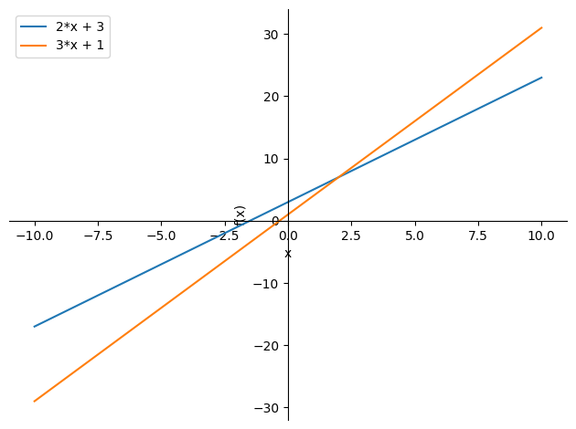
We use the plot() function with the equations for the two lines but also pass two additional keyword arguments — legend. By setting the legend argument to True, we add a legend to the graph. p[0] refers to the first line, \(2x + 3\), and we set its line_color attribute to 'b', indicating that we want this line to be blue. Similarly, we set the color of the second plot to red using the string 'r'.
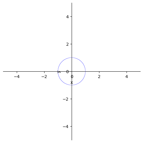
You can even plot an implicit function using plot_implicit() function. For example, let’s plot the circle \(x^2 + y^2 = 1\):
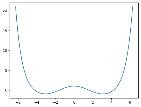
11.5.1 Exercise 2: Find all the intersection points between \(f(x)=4\cos(3x)\) and \(g(x)=x^3\) using
SymPyby first plotting the function and using the graph to narrow down the range of the intersection points. Then, usensolve()function to find the intersection points.
Hint: You may find solve() and nroots() can not be used to solve this problem. In addition, you may need to zoom in around 0 to find all the possible intersection points.
SymPySymPy is also capable of calculating the Taylor series of an expression at a specific point. Utilize series(expr, x, x0, n) to determine the series expansion of expr around the point x = x0 up to O(x^n) (where n is an integer):
\(\displaystyle 1 - \frac{x^{2}}{2} + \frac{x^{4}}{24} - \frac{x^{6}}{720} + \frac{x^{8}}{40320} + O\left(x^{10}\right)\)
\(\displaystyle \frac{x^{9}}{362880} - \frac{x^{7}}{5040} + \frac{x^{5}}{120} - \frac{x^{3}}{6} + x\)
Additionally, we can eliminate the O(x^n) term by applying the removeO() method:
lambdify()The lambdify() function translates SymPy expressions into Python functions so that they can be evaluated numerically.
\(\displaystyle 1.0\)
To find limits of functions in SymPy, we can create objects of the Limit class as follows:
\(\displaystyle \lim_{x \to \infty} \frac{1}{x}\)
The result is returned as an unevaluated object. To obtain the value of the limit, we can use the doit() method:
By default, the limit is calculated from a positive direction unless the value at which the limit is to be computed is positive or negative infinity. If the limit is at positive infinity, the direction is negative, and if it is at negative infinity, the direction is positive. We can change the default direction as follows:
sp.Limit(1/x, x, 0).doit(), sp.Limit(1/x, x, 0, dir='+').doit(), sp.Limit(1/x, x, 0, dir='-').doit()\(\displaystyle \left( \infty, \ \infty, \ -\infty\right)\)
We can change the default direction of limit calculation using the dir argument. The symbol dir='-' specifies that we are approaching the limit from the negative side. Alternatively, instead of using the Limit class, we can use the limit() function to find the limit of a function directly:
To find the derivative of a function, we can create an object of Derivative class:
\(\displaystyle \frac{d}{d t} \left(5 t^{2} + 2 t + 8\right)\)
Similar to the Limit class, when we create an object of Derivative class, it doesn’t calculate the derivative right away. Instead, we need to call the doit() method on the unevaluated Derivative object to evaluate and obtain the derivative:
If we want to calculate the value of the derivative at a specific value of \(t\) such as \(t = t_1\) or \(t = 1\), we can use our subs() method:
\(\displaystyle \left( 10 t_{1} + 2, \ 12\right)\)
Similarly, we can also use the diff() function to find the derivative of a function directly:
To calculate higher derivatives, we can provide the third argument to specify the order:
We can determine either the indefinite integral (antiderivative) or the definite integral by generating an Integral object:
Just as with the Limit and Derivative classes, we can evaluate the integral by employing the doit() method:
Additionally, the integrate() function can be utilized to directly compute the integral of a given function:
\(\displaystyle \left( - \cos{\left(x \right)}, \ x \log{\left(x \right)} - x\right)\)
Again, it’s important to note that we should use the elementary math functions
sin()andlog()from theSymPylibrary in the above expression, rather than from alternative libraries such asNumPy.
To calculate the definite integral, we just need to provide the variable (symbol), the lower limit, and the upper limit as a tuple:
# sp.Integral(sp.sin(x), (x, 0, sp.pi / 2)).doit()
sp.integrate(sp.sin(x), (x, 0, sp.pi / 2)) # (function, (integration_variable, lower_limit, upper_limit))
\(\displaystyle 1\)
Improper integrals are supported as well:
SymPyMatrices can be generated as instances of the Matrix class:
When creating a matrix in SymPy, the syntax resembles that of NumPy: you supply a list of lists, with each list representing a row in the matrix:
\(\displaystyle \left[\begin{matrix}a & b & c\\x & y & z\\a & b & c\end{matrix}\right]\)
A matrix with a, b, c as diagonal elements can be constructed utilizing the diag() function:
\(\displaystyle \left[\begin{matrix}a & 0 & 0\\0 & b & 0\\0 & 0 & c\end{matrix}\right]\)
Matrix multiplication can then be performed using the * operator:
\(\displaystyle \left[\begin{matrix}a^{2} & b^{2} & c^{2}\\a x & b y & c z\\a^{2} & b^{2} & c^{2}\end{matrix}\right]\)
Scalar multiplication and addition function as anticipated:
\(\displaystyle \left[\begin{matrix}4 a & 3 b & 3 c\\3 x & b + 3 y & 3 z\\3 a & 3 b & 4 c\end{matrix}\right]\)
The inverse of the matrix can be acquired using the inv() method:
\(\displaystyle \left[\begin{matrix}\frac{1}{a} & 0 & 0\\0 & \frac{1}{b} & 0\\0 & 0 & \frac{1}{c}\end{matrix}\right]\)
The matrix’s eigenvalues and eigenvectors can be derived using the eigenvals() and eigenvects() methods:
\(\displaystyle \left( \left\{ a : 1, \ b : 1, \ c : 1\right\}, \ \left[ \left( a, \ 1, \ \left[ \left[\begin{matrix}1\\0\\0\end{matrix}\right]\right]\right), \ \left( b, \ 1, \ \left[ \left[\begin{matrix}0\\1\\0\end{matrix}\right]\right]\right), \ \left( c, \ 1, \ \left[ \left[\begin{matrix}0\\0\\1\end{matrix}\right]\right]\right)\right]\right)\)
If you would like more information about the Matrix class and linear algebra with SymPy, refer to the official documentation.
You can also explore the Sympy Gamma and SymPy Live websites to learn more about SymPy.
All in all, SymPy is a Python library for symbolic mathematics. It aims to provide a computer algebra system that is both easy to use and extensible. Unlike numerical libraries, which focus on approximations and numerical computations, SymPy is designed to perform algebraic manipulations and simplifications symbolically, allowing for exact solutions to mathematical problems.
SymPy offers a wide range of features, including basic arithmetic operations, algebraic manipulation, calculus, equation solving, linear algebra, and more. It is particularly well-suited for tasks that require manipulation of symbolic expressions or solving equations symbolically.