stuff = list()
stuff.append('python')
stuff.append('chuck')
stuff.sort()
print(stuff[0])
print(stuff.__getitem__(0))
print(list.__getitem__(stuff,0))
chuck
chuck
chuck|
|

|
A data structure uses a collection of related variables that can be accessed individually or as a whole.
In other words, a data structure represents a set of data items that share a specific relationship.
As it turns out, we have been using objects. Python provides us with many built-in objects. Here is some simple code where the first few lines should feel very simple and natural to you.
stuff = list()
stuff.append('python')
stuff.append('chuck')
stuff.sort()
print(stuff[0])
print(stuff.__getitem__(0))
print(list.__getitem__(stuff,0))chuck
chuck
chuckThe first line constructs an object of type list, the second and third lines call the append() method, the fourth line calls the sort() method, and the fifth line retrieves the item at position 0. The sixth line calls the __getitem__() method in the stuff list with a parameter of zero. The seventh line is an even more verbose way of retrieving the 0th item in the list. In this code, we call the __getitem__ method in the list class and pass the list and the item we want retrieved from the list as parameters.
We can take a look at the capabilities of an object by looking at the output of the dir() function:
['__add__',
 '__class__',
 '__contains__',
 '__delattr__',
 '__delitem__',
 '__dir__',
 '__doc__',
 '__eq__',
 '__format__',
 '__ge__',
 '__getattribute__',
 '__getitem__',
 '__gt__',
 '__hash__',
 '__iadd__',
 '__imul__',
 '__init__',
 '__init_subclass__',
 '__iter__',
 '__le__',
 '__len__',
 '__lt__',
 '__mul__',
 '__ne__',
 '__new__',
 '__reduce__',
 '__reduce_ex__',
 '__repr__',
 '__reversed__',
 '__rmul__',
 '__setattr__',
 '__setitem__',
 '__sizeof__',
 '__str__',
 '__subclasshook__',
 'append',
 'clear',
 'copy',
 'count',
 'extend',
 'index',
 'insert',
 'pop',
 'remove',
 'reverse',
 'sort']
An object can contain a number of functions (which we call methods) as well as data that is used by those functions. We call data items that are part of the object attributes.
We use the class keyword to define the data and code that will make up each of the objects. The class keyword includes the name of the class and begins an indented block of code where we include the attributes (data) and methods (code).
class PartyAnimal:
   x = 0

   def party(self) :
     self.x = self.x + 1
     print("So far",self.x)

an = PartyAnimal()
an.party()
an.party()
an.party()
So far 1
So far 2
So far 3Each method looks like a function, starting with the def keyword and consisting of an indented block of code. This object has one attribute (x) and one method (party). The methods have a special first parameter that we name by convention self.
Just as the def keyword does not cause function code to be executed, the class keyword does not create an object. We need instruct Python to construct (i.e., create) an object or instance of the class PartyAnimal. It looks like a function call to the class itself. Python constructs the object with the right data and methods and returns the object which is then assigned to the variable an
When the PartyAnimal class is used to construct an object, the variable an is used to point to that object. We use an to access the code and data for that particular instance of the PartyAnimal class.
Each Partyanimal object/instance contains within it a variable x and a method/function named party. We call the party method in this line:
When the party method is called, the first parameter (which we call by convention self) points to the particular instance of the PartyAnimal object that party is called from. Within the party method, we see the line:
This syntax using the dot operator is saying ‘the x within self.’ Each time party() is called, the internal x value is incremented by 1 and the value is printed out.
In the previous examples, we define a class (template), use that class to create an instance of that class (object), and then use the instance. When the program finishes, all of the variables are discarded. Usually, we don’t think much about the creation and destruction of variables, but often as our objects become more complex, we need to take some action within the object to set things up as the object is constructed and possibly clean things up as the object is discarded.
If we want our object to be aware of these moments of construction and destruction, we add specially named methods to our object:
class PartyAnimal:
   def __init__(self):
     self.x = 0
     print('I am constructed')

   def party(self, y=5): # We can pass parameter like this
     self.x = self.x + y
     print('So far',self.x)

   def __del__(self):
     print('I am destructed', self.x)

an = PartyAnimal()
an.party()
an.party(10)
an.party(10)
an = 42
print('an contains',an)
I am constructed
So far 5
So far 15
So far 25
I am destructed 25
an contains 42As Python constructs our object, it calls our __init__ method to give us a chance to set up some default or initial values for the object. When Python encounters the line:
It actually “throws our object away” so it can reuse the an variable to store the value 42. Just at the moment when our an object is being “destroyed” our destructor code (__del__) is called. We cannot stop our variable from being destroyed, but we can do any necessary cleanup right before our object no longer exists.
To process large amounts of data, we need a data structure such as an array. An array is a sequenced collection of elements, of the same data type. We can refer to the elements in the array as the first element, the second element, and so forth until we get to the last element.
If we were to put our 100 scores into an array, we could designate the elements as scores[0], scores[1], and so on. The index indicates the ordinal number of the element, counting from the beginning of the array. The array as a whole has a name, scores, but each score can be accessed individually using its subscript as follows:
Because arrays store information in adjoining blocks of memory, they’re considered contiguous data structures. In Python, we can use list or array from numpy library to implement array. See here for more information.
Python list: - Python lists are very general. They can contain any kind of object and are dynamically typed - However, they do not support mathematical functions such as matrix and dot multiplications. Implementing such functions for Python lists would not be very efficient because of the dynamic typing
NumPy array: - Extension package to Python for multi-dimensional arrays - Numpy arrays are statically typed and homogeneous. The type of the elements is determined when the array is created - Because of the static typing, fast implementation of mathematical functions such as multiplication and addition of numpy arrays can be implemented in a compiled language (C and Fortran is used). Moreover, Numpy arrays are memory efficient
A string can be considered as an array of characters, see here.
The numpy package (module) is used in almost all numerical computation using Python. It is a package that provides high-performance vector, matrix and higher-dimensional data structures for Python. It is implemented in C and Fortran so when calculations are vectorized (formulated with vectors and matrices) it can provides good performance
You can easily create 1D array (Vector) using a Python list
# a vector: the argument to the array function is a Python list
v = np.array([1,2,3,4])
v, type(v), v.dtype, v.shape
(array([1, 2, 3, 4]), numpy.ndarray, dtype('int64'), (4,))D.3.1.1 Example 1: Try to compare the speed of increment an array of integers containing 0 to 9999 by 1 using python list and numpy array.
start = timer()
# Your code here
for i in range(10000):
  a[i] = a[i]+1
end = timer()
print("Total time : %.3f ms" % (10**3 * (end - start)))
Total time : 2.783 msTotal time : 0.169 msThe arrays discussed so far are known as one-dimensional arrays because the data is organized linearly in only one direction. Many applications require that data be stored in more than one dimension. One common example is a table, which is an array that consists of rows and columns. The following figure shows a table, which is commonly called a two-dimensional array (Matrix).
The array shown below holds the scores of students in a class. There are five students in the class and each student has four different scores for four subjects. The variable scores[2][3] show the score of the second student in the third quiz. Arranging the scores in a two-dimensional array can help us to find the average of scores for each student (the average over the row values) and find the average for each subject (the average over the column values), as well as the average of all subjects (the average of the whole table). Note that multidimensional arrays — arrays with more than two dimensions — are also possible.
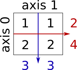
# a matrix: the argument to the array function is a nested Python list
M = np.array([[1, 1], [2, 2]]) # You can use nested list to implement 2D array in Python
M, type(M), M.dtype, M.shape
(array([[1, 1],
[2, 2]]), numpy.ndarray, dtype('int64'), (2, 2))Note the slicing of array works the same way as python list!
The indexes in a one-dimensional array directly define the relative positions of the element in actual memory. A two-dimensional array, however, represents rows and columns. How each element is stored in memory depends on the computer. Most computers use row-major storage, in which an entire row of an array is stored in memory before the next row. However, a computer may store the array using column-major storage, in which the entire column is stored before the next column. The following figure shows a two-dimensional array and how it is stored in memory using row-major or column-major storage. Row-major storage is more common.
By default, numpy array are row-major (C_CONTIGUOUS)
  C_CONTIGUOUS : True
  F_CONTIGUOUS : False
  OWNDATA : True
  WRITEABLE : True
  ALIGNED : True
  WRITEBACKIFCOPY : False
  UPDATEIFCOPY : False
You can change to column major (F_CONTIGUOUS) but it will be much slower in numpy due to the cache effect (functions in numpy assumes that the array are stored in column major)
  C_CONTIGUOUS : False
  F_CONTIGUOUS : True
  OWNDATA : True
  WRITEABLE : True
  ALIGNED : True
  WRITEBACKIFCOPY : False
  UPDATEIFCOPY : False
D.3.3.1 Exercise 1: We have stored the two-dimensional array students in the memory. The array is 100 × 4 (100 rows and 4 columns). Show the address of the element
students[5][3]assuming that the elementstudent[0][0]is stored in the memory location with address 0 and each element occupies only one memory location. The computer uses row-major storage.
We can use the following formula to find the location of an element, assuming each element occupies one memory location:
\(y = x + Cols \times i + j\)
where x defines the start address, Cols defines the number of columns in the array, i defines the row number of the element, j defines the column number of the element, and y is the address we are looking for. In our example, x is 0, Cols is 4, i is 5 and j is 3. We are looking for the value of y:
\(y = 0 + 4 \times i + j = 23\)
Traditionally, computer languages require that the size of an array (the number of elements in the array) be defined at the time the program is written and prevent it from being changed during the execution of the program. Recently, some languages have allowed variable-size arrays. Even when the language allows variable-sized arrays, insertion of an element into an array needs careful attention! See here for more information.
Both
listandarraycan be considered as dynamic array
We often need to find the index of an element when we know the value. This type of search was discussed in Chapter 8. We can use sequential search for unsorted arrays or binary search on sorted arrays
If the insertion is at the end of an array this can be done easily. For example, if an array has 30 elements, we increase the size of the array to 31 and insert the new item as the 31st item.
[1, 2, 3, 4, 5, 6, 7, 8, 9, 10, 11, 12, 13, 14, 15, 16, 17, 18, 19, 20, 21, 22, 23, 24, 25, 26, 27, 28, 29, 30, 31]If the insertion is to be at the beginning or in the middle of an array, the process is lengthy and time consuming. For example, if we want to insert an element as the 9th element in an array of 30 elements, elements 9 to 30 should be shifted one element towards the end of the array to open an empty element at position 9 for insertion. The following shows
D.3.4.4 Example 2: Try to insertion an element 31 as the 9th element in an array of 30 elements.
Elements 9 to 30 should be shifted one element towards the end of the array to open an empty element at position 9 for insertion. The following shows how to do it:
[ 1  2  3  4  5  6  7  8  9 10 11 12 13 14 15 16 17 18 19 20 21 22 23 24
 25 26 27 28 29 30]
i = 30
student = np.append(student,0) # Need to enlarge the space of array first!
while(i>=9):
student[i] = student[i-1]
i = i-1
student[i] = 31
print(student)[ 1 2 3 4 5 6 7 8 31 9 10 11 12 13 14 15 16 17 18 19 20 21 22 23
24 25 26 27 28 29 30]Note that the shifting needs to take place from the end of the array to prevent losing the values of the elements. The code first copies the value of the 30th element into the 31st element, then copies the value of the 29th element into the 30th element, and so on. When the code comes out of the loop, the 9th element is already copied to the 10th element. The last line copies the value of the new item into the 9th element.
Deletion of an element in an array is as lengthy and involved as insertion. For example, if the ninth element should be deleted, we need to shift elements 10 to 30 one position towards the start of the array.
D.3.5.1 Exercise 2: Try to delete an the element in the 9th position of an array of 30 elements.
[ 1  2  3  4  5  6  7  8  9 10 11 12 13 14 15 16 17 18 19 20 21 22 23 24
 25 26 27 28 29 30]
We need to shift elements 10 to 30 one position towards the start of the array
[ 1  2  3  4  5  6  7  8 10 11 12 13 14 15 16 17 18 19 20 21 22 23 24 25
26 27 28 29 30 30]an array is a random-access structure, which means that each element of an array can be accessed randomly without the need to access the elements before or after it.
Array traversal refers to an operation that is applied to all elements of the array, such as reading, writing, applying mathematical operation, and so on. You can use loop like list but vectorization usually works better as we have seen earlier.
An array is a suitable structure when a small number of insertions and deletions are required, but a lot of searching and retrieval is needed.
A record is a collection of related elements, possibly of different types, having a single name. Each element in a record is called a field. A field differs from a variable primarily in that it is part of a record. The following figure contains two examples of records. The first example, fraction, has two fields, both of which are integers. The second example, student, has three fields made up of three different types.
The elements in a record can be of the same or different types, but all elements in the record must be related.
Using dictionaries as a record data type or data object in Python is possible. Dictionaries are easy to create in Python as they have their own syntactic sugar built into the language.
The name of the record is the name of the whole structure, while the name of each field allows us to refer to that field. For example, in the student record of previous Figure, the name of the record is student, the name of the fields are student["id"], student["name"], and student["grade"].
Some programming languages use a period (.) to separate the name of the structure (record) from the name of its components (fields). You can implement this in Python using the following class.
We can conceptually compare an array with a record. This helps us to understand when we should use an array and when a record. An array defines a combination of elements, while a record defines the identifiable parts of an element. For example, an array can define a class of students (40 students), but a record defines different attributes of a student, such as id, name, or grade.
If we need to define a combination of element and at the same time some attributes of each element, we can use an array of records. For example, in a class of 30 students, we can have an array of 30 records, each record representing a student. The following figure shows an array of 30 student records called students.
[{'id': 2000, 'name': 'Bob0', 'grade': 'A'},
 {'id': 2001, 'name': 'Bob1', 'grade': 'A'},
 {'id': 2002, 'name': 'Bob2', 'grade': 'A'},
 {'id': 2003, 'name': 'Bob3', 'grade': 'A'},
 {'id': 2004, 'name': 'Bob4', 'grade': 'A'},
 {'id': 2005, 'name': 'Bob5', 'grade': 'A'},
 {'id': 2006, 'name': 'Bob6', 'grade': 'A'},
 {'id': 2007, 'name': 'Bob7', 'grade': 'A'},
 {'id': 2008, 'name': 'Bob8', 'grade': 'A'},
 {'id': 2009, 'name': 'Bob9', 'grade': 'A'},
 {'id': 2010, 'name': 'Bob10', 'grade': 'A'},
 {'id': 2011, 'name': 'Bob11', 'grade': 'A'},
 {'id': 2012, 'name': 'Bob12', 'grade': 'A'},
 {'id': 2013, 'name': 'Bob13', 'grade': 'A'},
 {'id': 2014, 'name': 'Bob14', 'grade': 'A'},
 {'id': 2015, 'name': 'Bob15', 'grade': 'A'},
 {'id': 2016, 'name': 'Bob16', 'grade': 'A'},
 {'id': 2017, 'name': 'Bob17', 'grade': 'A'},
 {'id': 2018, 'name': 'Bob18', 'grade': 'A'},
 {'id': 2019, 'name': 'Bob19', 'grade': 'A'},
 {'id': 2020, 'name': 'Bob20', 'grade': 'A'},
 {'id': 2021, 'name': 'Bob21', 'grade': 'A'},
 {'id': 2022, 'name': 'Bob22', 'grade': 'A'},
 {'id': 2023, 'name': 'Bob23', 'grade': 'A'},
 {'id': 2024, 'name': 'Bob24', 'grade': 'A'},
 {'id': 2025, 'name': 'Bob25', 'grade': 'A'},
 {'id': 2026, 'name': 'Bob26', 'grade': 'A'},
 {'id': 2027, 'name': 'Bob27', 'grade': 'A'},
 {'id': 2028, 'name': 'Bob28', 'grade': 'A'},
 {'id': 2029, 'name': 'Bob29', 'grade': 'A'}]
In an array of records, the name of the array defines the whole structure, the group of students as a whole. To define each element, we need to use the corresponding index. To define the parts (attributes) of each element, we need to use the dot operator. In other words, first we need to define the element, then we can define part of that element. Therefore, the id of the third student is defined as:
Both an array and an array of record represents a list of items. An array can be thought of as a special case of an array of records in which each element is a record with only a single field!
A linked list is a collection of data in which each element contains the location of the next element — that is, each element contains two parts: data and link. The data part holds the value information: the data to be processed. The link is used to chain the data together, and contains a pointer (an address) that identifies the next element in the list. In addition, a pointer variable identifies the first element in the list. The name of the list is the same as the name of the first pointer variable.
The following figure shows a linked list called scores that contains four elements. The link in each element, except the last, points to its successor. The link in the last element contains a null pointer, indicating the end of the list. We define an empty linked list to be only a null pointer:
The elements in a linked list are traditionally called nodes. A node in a linked list is a record that has at least two fields: one contains the data, and the other contains the address of the next node in the sequence (the link).
Before further discussion of linked lists, we need to explain the notation we use in the figures. We show the connection between two nodes using a line. One end of the line has an arrowhead, the other end has a solid circle. The arrowhead represents a copy of the address of the node to which the arrow head is pointed. The solid circle shows where this copy of the address is stored. The figure also shows that we can store a copy of the address in more than one place!
Both an array and a linked list are representations of a list of items in memory. The only difference is the way in which the items are linked together. In an array of records, the linking tool is the index. The element scores[3] is linked to the element scores[4] because the integer 4 comes after the integer 3. In a linked list, the linking tool is the link that points to the next element — the pointer or the address of the next element.
The list is contiguous. The nodes of a linked list can be stored with gaps between them: the link part of the node ‘glues’ the items together. In other words, the computer has the option to store them contiguously or spread the nodes through the whole memory. This has an advantage: insertion and deletion in a linked list is much easier. The only thing that needs to be changed is the pointer to the address of the next element. However, this comes with an overhead: each node of a linked list has an extra field, the address of the next node in memory.
In Python, there’s a specific object in the collections module that you can use for linked lists called deque (pronounced “deck”), which stands for double-ended queue.
https://realpython.com/linked-lists-python/
But we can create a linked list using custom class in order to help our understanding! First things first, create a class to represent your linked list:
The only information you need to store for a linked list is where the list starts (the head of the list). Next, create another class to represent each node of the linked list:
In the above class definition, you can see the two main elements of every single node: data and link.
second_node = Node(72)
third_node = Node(96)
first_node.link = second_node
second_node.link = third_node
score
66 -> 72 -> 96 -> NoneBy defining a node’s data and link values, you can create a linked list quite quickly. Here’s a slight change to the linked list’s __init__() that allows you to quickly create linked lists with some data:
class LinkedList:
  def __init__(self, nodes=None):
    self.head = None
    if nodes:
      node = Node(data=nodes.pop(0)) #pop will pop out the first entry of the list
      self.head = node
      for elem in nodes:
        node.link = Node(data=elem)
        node = node.link
  def __repr__(self): #This is to beautify printing, don't worry about this
    node = self.head
    nodes = []
    while node is not None:
      nodes.append(str(node.data))
      node = node.link
    nodes.append("None")
return " -> ".join(nodes)The same operations we defined for an array can be applied to a linked list.
The search algorithm for a linked list can only be sequential (see Chapter 8) because the nodes in a linked list have no specific names (unlike the elements in an array) that can be found using a binary search. Since nodes in a linked list have no names, we use two pointers, pre (for previous) and cur (for current).
At the beginning of the search, the pre pointer is null and the cur pointer points to the first node. The search algorithm moves the two pointers together towards the end of the list. The following figure shows the movement of these two pointers through the list in an extreme case scenario: when the target value is larger than any value in the list. For example, in the five-node list, assume that our target value is 220, which is larger than any value in the list.
When the search stops, the cur pointer points to the node that stops the search and the pre pointer points to the previous node. If the target is found, the cur pointer points to the node that holds the target value. If the target value is not found, the cur pointer points to the node with a value larger than the target value. In other words, since the list is sorted, and may be very long, we never allow the two pointers to reach the end of the list if we are sure that we have passed the target value. The searching algorithm uses a flag (a variable that can take only true or false values). When the target is found, the flag is set to true: when the target is not found, the flag is set to false. When the flag is true the cur pointer points to the target value: when the flag is false, the cur pointer points to a value larger than the target value.
The following shows some different situations. In the first case, the target is 98. This value does not exist in the list and is smaller than any value in the list, so the search algorithm stops while pre is null and cur points to the first node. The value of the flag is false because the value was not found. In the second case, the target is 132, which is the value of the second node. The search algorithm stops while cur is pointing to the second node and pre is pointing to the first node. The value of the flag is true because the target is found. In the third and the fourth cases, the targets are not found so the value of the flag is false.
D.5.3.2 Example 3: The following shows a simplified algorithm for the search. Note how
we move the two pointers forward together. This guarantees that the two pointers move together. The search algorithm is used both by the insertion algorithm (if the target is not found) and by the delete algorithm (if the target is found).
def SearchLinkedList(ilist, target):
  """
    Parameters
    ----------
    numbers: ilist
        The input list.
    target: int
        The target value.
    Returns
    -------
    cur : Node
        The current pointer
    pre : Node
        The pre pointer
    flag : bool
        Whether the taget had been found or not
  """
  # Your code here
  pre = None
  cur = ilist.head
  while(cur!=None and target > cur.data):
    pre = cur
    cur = cur.link
  if cur!=None and cur.data == target:
    flag = True
  else:
    flag = False
return cur, pre, flagBefore insertion into a linked list, we first apply the searching algorithm. If the flag returned from the searching algorithm is false, we will allow insertion, otherwise we abort the insertion algorithm, because we do not allow data with duplicate values. Four cases can arise:
If the list is empty (ilist = None), the new item is inserted as the first element. One statement can do the job:
If the searching algorithm returns a flag with value of false and the value of the pre pointer is null, the data needs to be inserted at the beginning of the list. Two statements are needed to do the job:
(102, None, False)The first assignment makes the new node become the predecessor of the previous first node. The second statement makes the newly connected node the first node.
If the searching algorithm returns a flag with value of false and the value of the cur pointer is null, the data needs to be inserted at the end of the list. Two statements are needed to do the job:
(None, 201, False)The first assignment connects the new node to the previous last node. The second statement makes the newly connected node become the last node.
If the searching algorithm returns a flag with a value of false and none of the returned pointers are null, the new data needs to be inserted at the middle of the list. Two statements are needed to do the job:
(178, 132, False)The first assignment connects the new node to its successor. The second statement connects the new node to its predecessor.
D.5.3.4 Exercise 3: The following shows the pseudocode for inserting a new node in a linked list. The first section just adds a node to an empty list.
def InsertLinkedList(ilist, target, new):
  """
    Parameters
    ----------
    ilist: llist
        The input list.
    target: int
        The target value.
    new: Node
        The node that should be inserted
    Returns
    -------
    ilist : llist
        The new linked list
  """
  # Your code here
  cur, pre, flag = SearchLinkedList(ilist, target)
  if flag == True:
    return ilist
  if ilist.head == None:
    new.data = target
    ilist.head = new
  elif pre == None:
    new.data = target
    new.link = cur
    ilist.head = new
  elif cur == None:
    new.data = target
    pre.link = new
    new.link = None
  else:
    new.data = target
    new.link = cur
    pre.link = new

return ilist95 -> 102 -> 132 -> 178 -> 201 -> None102 -> 132 -> 178 -> 201 -> 220 -> NoneBefore deleting a node in a linked list, we apply the search algorithm. If the flag returned from the search algorithm is true (the node is found), we can delete the node from the linked list. However, deletion is simpler than insertion: we have only two cases — deleting the first node and deleting any other node. In other words, the deletion of the last and the middle nodes can be done by the same process.
If the pre pointer is null, the first node is to be deleted. The cur pointer points to the first node and deleting can be done by one statement:
(102, None, True)The statement connects the second node to the list pointer, which means that the first node is deleted.
If neither of the pointers is null, the node to be deleted is either a middle node or the last node. The cur pointer points to the corresponding node and deleting can be done by one statement:
(132, 102, True)(201, 178, True)The statement connects the successor node to the predecessor node, which means that the current node is deleted.
D.5.3.6 Exercise 4: The following algorithm shows the pseudocode for deleting a node. The algorithm is much simpler than the one for inserting. We have only two cases and each case needs only one statement.
def DeleteLinkedList(ilist, target):
  """
    Parameters
    ----------
    ilist: llist
        The input list.
    target: int
        The target value.
    Returns
    -------
    ilist : llist
        The new linked list
  """
  # Your code here
  cur, pre, flag = SearchLinkedList(ilist, target)
  if flag == False:
    return ilist
  elif pre == None:
    ilist.head = cur.link
  else:
    pre.link = cur.link
return ilistRetrieving means randomly accessing a node for the purpose of inspecting or copying the data contained in the node. Before retrieving, the linked list needs to be searched. If the data item is found, it is retrieved, otherwise the process is aborted. Retrieving uses only the cur pointer, which points to the node found by the search algorithm.
D.5.3.8 Example 4:

To traverse the list, we need a ‘walking’ pointer, which is a pointer that moves from node to node as each element is processed. We start traversing by setting the walking pointer to the first node in the list. Then, using a loop, we continue until all of the data has been processed. Each iteration of the loop processes the current node, then advances the walking pointer to the next node. When the last node has been processed, the walking pointer becomes null and the loop terminates.
D.5.3.10 Example 5:

A linked list is a very efficient data structure for storing data that will go through many insertions and deletions. A linked list is a dynamic data structure in which the list can start with no nodes and then grow as new nodes are needed. A node can be easily deleted without moving other nodes, as would be the case with an array. For example, a linked list could be used to hold the records of students in a school. Each quarter or semester, new students enroll in the school and some students leave or graduate.
A linked list can grow infinitely and can shrink to an empty list. The overhead is to hold an extra field for each node. A linked list, however, is not a good candidate for data that must be searched often. This appears to be a dilemma, because each deletion or insertion needs a search. We will see that some abstract data types, discussed in the next chapter, have the advantages of an array for searching and the advantages of a link list for insertion and deletion.
A linked list is a suitable structure if a large number of insertions and deletions are needed, but searching a linked list is slower that searching an array.