Trees and Tree Algorithms

!pip install jupyterquiz 
!pip install jupytercards

from IPython.display import display, Javascript
display(Javascript('Jupyter.notebook.kernel.restart()'))

Requirement already satisfied: jupyterquiz in /home/phonchi/miniconda3/lib/python3.13/site-packages (2.9.6.4)

Requirement already satisfied: jupytercards in /home/phonchi/miniconda3/lib/python3.13/site-packages (3.2.1)

from jupyterquiz import display_quiz

path="https://raw.githubusercontent.com/phonchi/nsysu-math208/refs/heads/main/extra/questions/ch9/"
#path="questions/ch9/"

# === DS09 animation infrastructure (run once before any animation cell). ===
# Self-contained: fetches the engine + per-animation markup from GitHub
# (raw.githubusercontent.com), no local "animations09/" folder required.
from urllib.request import urlopen
from functools import lru_cache
from IPython.display import HTML, display

_BASE = "https://raw.githubusercontent.com/phonchi/nsysu-math208/refs/heads/main/extra/animations09/"

@lru_cache(maxsize=32)
def _fetch(name):
    return urlopen(_BASE + name, timeout=15).read().decode("utf-8")

def load_infra():
    display(HTML("<style>" + _fetch("ds09.css") + "</style>"
                 "<script>" + _fetch("ds09.js") + "</script>"))

def load_anim(name):
    display(HTML(_fetch(name + ".html")))

_ = load_infra()

1. The Tree Abstract Data Type

2. Tree Traversals

3. Priority Queue and Binary Heap

4. Binary Search Trees

5. AVL tree

6.2 Introduction

Trees are used in many areas of computer science, including operating systems, graphics, database systems, and computer networking. A tree data structure has a root, branches, and leaves. The difference between a tree in nature and a tree in computer science is that a tree data structure has its root at the top and its leaves on the bottom!

Our first example of a tree is a classification tree from biology which shows an example of the biological classification of some animals.

This example demonstrates that trees are hierarchical. By hierarchical, we mean that trees are structured in layers with the more general things near the top and the more specific things near the bottom. The top of the hierarchy is the kingdom, the next layer of the tree (the "children" of the layer above) is the phylum, then the class, and so on.

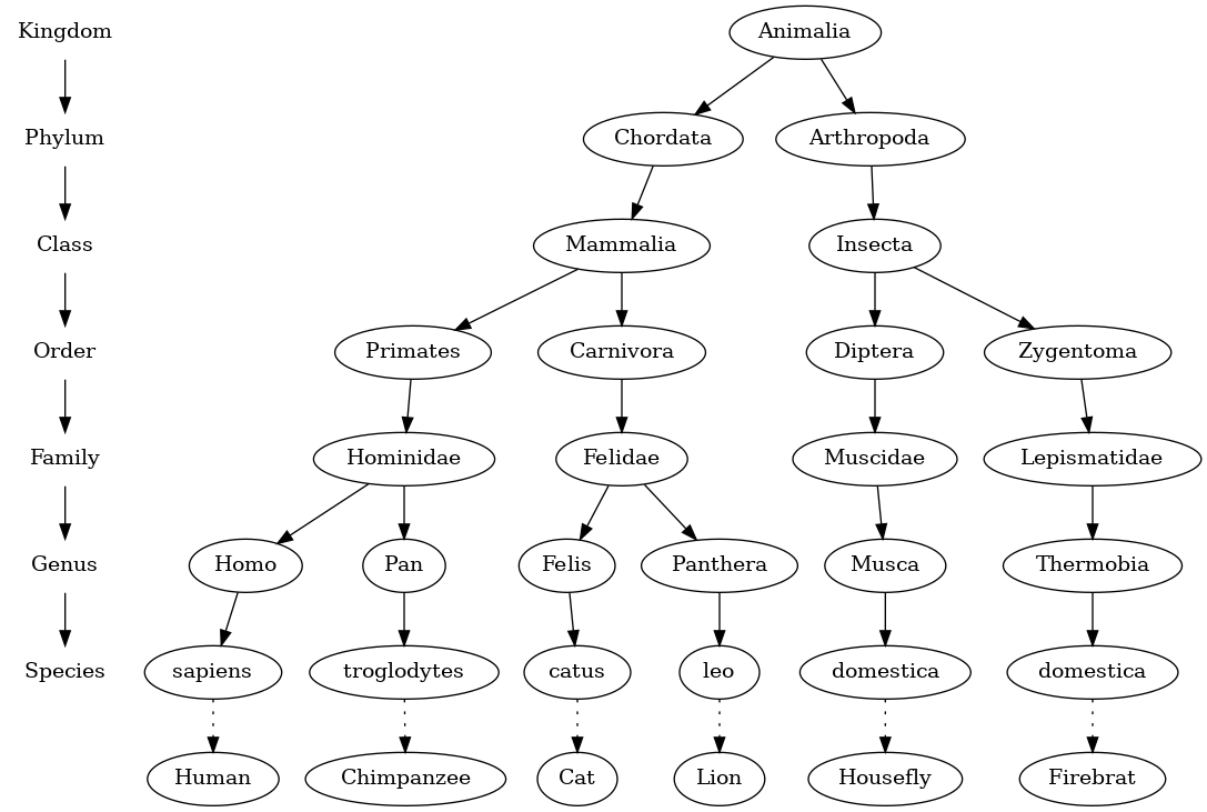
Notice that you can start at the top of the tree and follow a path made of circles and arrows all the way to the bottom. At each level of the tree we might ask ourselves a question and then follow the path that agrees with our answer.

For example we might ask, "Is this animal a chordate or an arthropod?" If the answer is "chordate," then we follow that path and ask, "Is this chordate a mammal?" If not, we are stuck (but only in this simplified example). When we are at the mammal level we ask, "Is this mammal a primate or a carnivore?" We can keep following paths until we get to the very bottom of the tree where we have the common name!

A second property of trees is that all of the children of one node are independent of the children of another node while the third property is that each leaf node is unique.

We can specify a path from the root of the tree to a leaf that uniquely identifies each species in the animal kingdom, for example Animalia -> Chordata -> Mammalia -> Carnivora -> Felidae -> Felis -> catus.

Another example of a tree structure that you probably use every day is a file system. In a file system, directories, or folders, are structured as a tree. The file system tree enables you to follow a path from the root to any directory. That path will uniquely identify that subdirectory

Note that we could take the entire subtree staring with /etc/, detach etc/ from the root and reattach it under usr/. This would change the unique pathname to httpd from /etc/httpd to /usr/etc/httpd, but would not affect the contents or any children of the httpd directory!

6.3. Vocabulary and Definitions

• Node: A node is a fundamental part of a tree. It can have a name, which we call the key. A node may also have additional information. We call this additional information the value or payload.

• Edge: An edge is another fundamental part of a tree. An edge connects two nodes to show that there is a relationship between them. Every node (except the root) is connected by exactly one incoming edge from another node. Each node may have several outgoing edges.

• Root: The root of the tree is the only node in the tree that has no incoming edges.

• Path: A path is an ordered list of nodes that are connected by edges, for example, Mammalia -> Carnivora -> Felidae -> Felis -> catus is a path.

• Children: The set of nodes that have incoming edges from the same node are said to be the children of that node.
• Parent: A node is the parent of all the nodes it connects to with outgoing edges.

• Sibling: Nodes in the tree that are children of the same parent are said to be siblings. The nodes etc/ and usr/ are siblings in the file system tree shown in Figure 2.
• Subtree: A subtree is a set of nodes and edges comprised of a parent and all the descendants of that parent.

• Leaf Node: A leaf node is a node that has no children.
• Level: The level of a node $n$ is the number of edges on the path from the root node to $n$.
• Height: The height of a tree is equal to the maximum level of any node in the tree.

Definition One: A tree consists of a set of nodes and a set of edges that connect pairs of nodes. A tree has the following properties:

1. One node of the tree is designated as the root node.

2. Every node $n$, except the root node, is connected by an edge from exactly one other node $p$, where $p$ is the parent of $n$.

3. A unique path traverses from the root to each node.

4. If each node in the tree has a maximum of two children, we say that the tree is a binary tree.

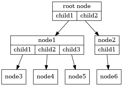
The arrowheads on the edges indicate the direction of the connection.

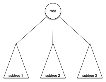
Definition Two: A tree is either empty or consists of a root and zero or more subtrees, each of which is also a tree. The root of each subtree is connected to the root of the parent tree by an edge.

Figure below illustrates this recursive definition of a tree. Using the recursive definition of a tree, we know that the tree below has at least four nodes (if it is not empty) since each of the triangles representing a subtree must have a root. It may have many more nodes than that, but we do not know unless we look deeper into the tree!

display_quiz(path+"tree.json", max_width=800)

6.4. Tree ADT

We can use the following functions to create and manipulate a binary tree:

• BinaryTree(): creates a new instance of a binary tree.

• get_root_val(): returns the value stored in the current node.

• set_root_val(val): stores the value in parameter val in the current node.

• get_left_child(): returns the binary tree corresponding to the left child of the current node.
• get_right_child(): returns the binary tree corresponding to the right child of the current node.

• insert_left(val): creates a new binary tree and installs it as the left child of the current node.

• insert_right(val): creates a new binary tree and installs it as the right child of the current node.

The key decision in implementing a tree is choosing a good internal storage technique. We have two very interesting possibilities, and we will examine both before choosing one. We call them list of lists and nodes and references.

6.5. List of Lists Representation

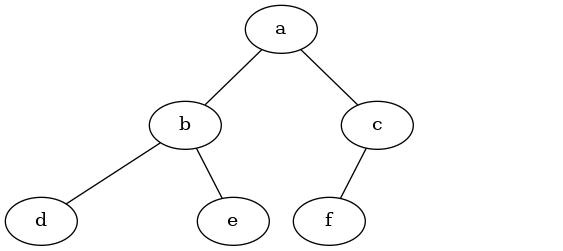
In a list of lists tree, we will store the value of the root node as the first element of the list. The second element of the list will itself be a list that represents the left subtree. The third element of the list will be another list that represents the right subtree. To illustrate this storage technique, let's look at an example. Figure below shows a simple tree and the corresponding list implementation:

my_tree = [
        "a",  # root
        ["b",  # left subtree
            ["d", [], []],
            ["e", [], []]
        ],
        ["c",  # right subtree
            ["f", [], []],
            []
        ],

Notice that we can access subtrees of the list using standard list indexing. The root of the tree is my_tree[0], the left subtree of the root is my_tree[1], and the right subtree is my_tree[2].

The structure of a list representing a subtree adheres to the structure defined for a tree; the structure itself is recursive! A subtree that has a root value and two empty lists is a leaf node. Another nice feature of the list of lists approach is that it generalizes to a tree that has many subtrees. In the case where the tree is more than a binary tree, another subtree is just another list!

my_tree = ["a", ["b", ["d", [], []], ["e", [], []]], ["c", ["f", [], []], []]]
print(my_tree)
print("left subtree = ", my_tree[1])
print("root = ", my_tree[0])
print("right subtree = ", my_tree[2])

['a', ['b', ['d', [], []], ['e', [], []]], ['c', ['f', [], []], []]]
left subtree =  ['b', ['d', [], []], ['e', [], []]]
root =  a
right subtree =  ['c', ['f', [], []], []]

Let's formalize this definition of the tree data structure by providing some functions that make it easy for us to use lists as trees. Note that we are not going to define a binary tree class. The functions we will write will just help us manipulate a standard list as though we are working with a tree!

def make_binary_tree(root):
    return [root, [], []]

def insert_left(root, new_child):
    old_child = root.pop(1)
    if len(old_child) > 1:
        root.insert(1, [new_child, old_child, []])
    else:
        root.insert(1, [new_child, [], []])
    return root

Notice that to insert a left child, we first obtain the (possibly empty) list that corresponds to the current left child. We then add the new left child, installing the old left child as the left child of the new one!

def insert_right(root, new_child):
    old_child = root.pop(2)
    if len(old_child) > 1:
        root.insert(2, [new_child, [], old_child])
    else:
        root.insert(2, [new_child, [], []])
    return root

def get_root_val(root):
    return root[0]
def set_root_val(root, new_value):
    root[0] = new_value

def get_left_child(root):
    return root[1]
def get_right_child(root):
    return root[2]

a_tree = make_binary_tree(3)
print(a_tree)
print(insert_left(a_tree, 4))
print(insert_left(a_tree, 5))
print(insert_right(a_tree, 6))

[3, [], []]
[3, [4, [], []], []]
[3, [5, [4, [], []], []], []]
[3, [5, [4, [], []], []], [6, [], []]]

6.6. Nodes and References

Our second method to represent a tree uses nodes and references. In this case we will define a class that has attributes for the root value as well as the left and right subtrees.

Using nodes and references, we might think of the tree as being structured like the one shown below:

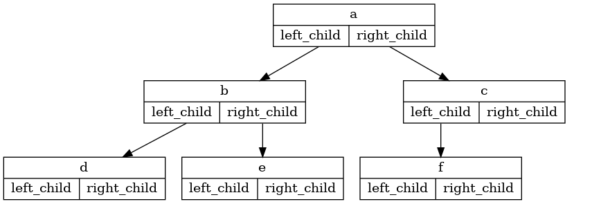
Since this representation more closely follows the object-oriented programming paradigm, we will continue to use this representation for the remainder of the chapter.

We will start out with a simple class definition for the nodes and references approach as shown below. The important thing to remember about this representation is that the attributes left_child and right_child will become references to other instances of the BinaryTree class. For example, when we insert a new left child into the tree, we create another instance of BinaryTree and modify self.left_child in the root to reference the new tree.

class BinaryTree:
    def __init__(self, root_obj):
        self.key = root_obj
        self.left_child = None
        self.right_child = None

Just as you can store any object you like in a list, the root object of a tree can be a reference to any object. For our early examples, we will store the name of the node as the root value. Using nodes and references to represent the tree above, we would create six instances of the BinaryTree class.

Next let's look at the functions we need to build the tree beyond the root node. To add a left child to the tree, we will create a new binary tree object and set the left_child attribute of the root to refer to this new object.

def insert_left(self, new_node):
    if self.left_child is None:
        self.left_child = BinaryTree(new_node)
    else:
        new_child = BinaryTree(new_node)
        new_child.left_child = self.left_child
        self.left_child = new_child

Note that we consider two cases for insertion. The first case is characterized by a node with no existing left child. When there is no left child, simply add a node to the tree. The second case is characterized by a node with an existing left child. In the second case, we insert a node and push the existing child down one level in the tree.

def insert_right(self, new_node):
    if self.right_child == None:
        self.right_child = BinaryTree(new_node)
    else:
        new_child = BinaryTree(new_node)
        new_child.right_child = self.right_child
        self.right_child = new_child

To round out the definition for a simple binary tree data structure, we will write accessor methods for the left and right children and for the root values:

def get_root_val(self):
    return self.key
def set_root_val(self, new_key):
    self.key = new_key

def get_left_child(self):
    return self.left_child
def get_right_child(self):
    return self.right_child

Now that we have all the pieces to create and manipulate a binary tree, let's use them to check on the structure a bit more. Let's make a simple tree with node a as the root, and add nodes "b" and "c" as children

import sys
sys.path.append("./pythonds3/")
from pythonds3.trees import BinaryTree

a_tree = BinaryTree("a")
print(a_tree.get_root_val())
print(a_tree.get_left_child())
a_tree.insert_left("b")
print(a_tree.get_left_child())
print(a_tree.get_left_child().get_root_val())
a_tree.insert_right("c")
print(a_tree.get_right_child())
print(a_tree.get_right_child().get_root_val())
a_tree.get_right_child().set_root_val("hello")
print(a_tree.get_right_child().get_root_val())

a
None
<pythonds3.trees.binary_tree.BinaryTree object at 0x7b698c717e10>
b
<pythonds3.trees.binary_tree.BinaryTree object at 0x7b698c7178d0>
c
hello

6.7. Parse Tree

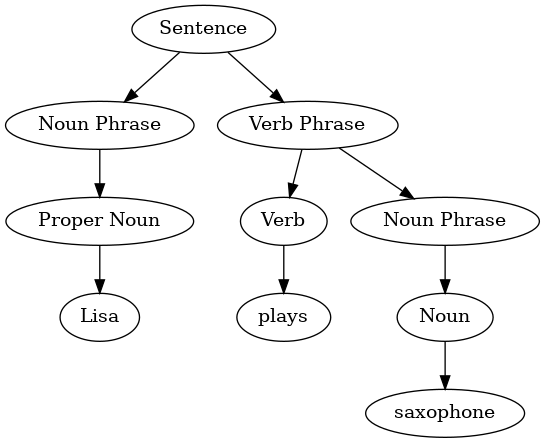
Parse trees can be used to represent real-world constructions like sentences or mathematical expressions. Figure below shows the hierarchical structure of a simple sentence. Representing a sentence as a tree structure allows us to work with the individual parts of the sentence by using subtrees.

We can also represent a mathematical expression such as $((7 + 3) \cdot (5 - 2))$ as a parse tree, as shown below:

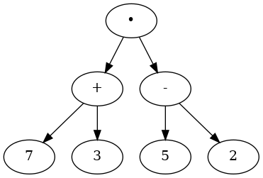
We know that multiplication has a higher precedence than either addition or subtraction. Because of the parentheses, we know that before we can do the multiplication we must evaluate the parenthesized addition and subtraction expressions. The hierarchy of the tree helps us understand the order of evaluation for the whole expression!

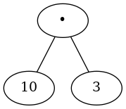
Before we can evaluate the top-level multiplication, we must evaluate the addition and the subtraction in the subtrees. The addition, which is the left subtree, evaluates to 10. The subtraction, which is the right subtree, evaluates to 3.

Using the hierarchical structure of trees, we can simply replace an entire subtree with one node once we have evaluated the expressions in the children. Applying this replacement procedure gives us the simplified tree shown below:

In the rest of this section we are going to examine parse trees in more detail. In particular we will look at

• How to build a parse tree from a fully parenthesized mathematical expression.

• How to evaluate the expression stored in a parse tree.

• How to recover the original mathematical expression from a parse tree.

The first step in building a parse tree is to break up the expression string into a list of tokens. There are four different kinds of tokens to consider: left parentheses, right parentheses, operators, and operands.

We know that whenever we read a left parenthesis we are starting a new expression, and hence we should create a new tree to correspond to that expression. Conversely, whenever we read a right parenthesis, we have finished an expression.

We also know that operands are going to be leaf nodes and children of their operators. Finally, we know that every operator is going to have both a left and a right child. Using the information from above we can define four rules as follows:

1. If the current token is a (, add a new node as the left child of the current node, and descend to the left child.

2. If the current token is in the list ["+", "-", "/", "*"], set the root value of the current node to the operator represented by the current token. Add a new node as the right child of the current node and descend to the right child.

3. If the current token is a number, set the root value of the current node to the number and return to the parent.

4. If the current token is a ), go to the parent of the current node.

Let's look at an example of the rules outlined above in action. We will use the expression $(3 + (4 * 5))$. We will parse this expression into the following list of character tokens: ["(", "3", "+", "(", "4", "*", "5", ")", ")"]. Initially we will start out with a parse tree that consists of an empty root node.

Figure below illustrates the structure and contents of the parse tree as each new token is processed:

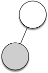
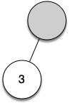
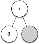
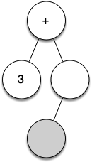
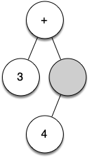
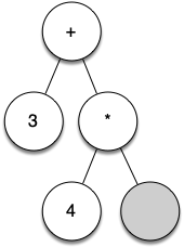
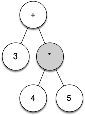
Let's walk through the example step by step:

1. Create an empty tree.

2. Read ( as the first token. By rule 1, create a new node as the left child of the root. Make the current node this new child.

3. Read 3 as the next token. By rule 3, set the root value of the current node to 3 and go back up the tree to the parent.

4. Read + as the next token. By rule 2, set the root value of the current node to + and add a new node as the right child. The new right child becomes the current node.

5. Read ( as the next token. By rule 1, create a new node as the left child of the current node. The new left child becomes the current node.

6. Read 4 as the next token. By rule 3, set the value of the current node to 4. Make the parent of 4 the current node.

7. Read * as the next token. By rule 2, set the root value of the current node to * and create a new right child. The new right child becomes the current node.

8. Read 5 as the next token. By rule 3, set the root value of the current node to 5. Make the parent of 5 the current node.

9. Read ) as the next token. By rule 4 we make the parent of * the current node.

10. Read ) as the next token. By rule 4 we make the parent of + the current node. At this point there is no parent for +, so we are done.

From the example above, it is clear that we need to keep track of the current node as well as the parent of the current node. The tree interface provides us with a way to get children of a node, through the get_left_child() and get_right_child() methods, but how can we keep track of the parent?

A simple solution to keeping track of parents as we traverse the tree is to use a stack. Whenever we want to descend to a child of the current node, we first push the current node on the stack. When we want to return to the parent of the current node, we pop the parent off the stack!

from pythonds3.basic import Stack
from pythonds3.trees import BinaryTree

def build_parse_tree(fp_expr):
    fp_list = fp_expr.split()
    p_stack = Stack()
    expr_tree = BinaryTree("")
    p_stack.push(expr_tree)
    current_tree = expr_tree

    for i in fp_list:
        if i == "(":
            current_tree.insert_left("")
            p_stack.push(current_tree)
            current_tree = current_tree.left_child
        elif i in ["+", "-", "*", "/"]:
            current_tree.root = i
            current_tree.insert_right("")
            p_stack.push(current_tree)
            current_tree = current_tree.right_child
        elif i.isdigit():
              current_tree.root = int(i)
              parent = p_stack.pop()
              current_tree = parent
        elif i == ")":
              current_tree = p_stack.pop()
        else:
              raise ValueError(f"Unknown operator '{i}'")
    return expr_tree

The four rules for building a parse tree are coded as the first four clauses of the if..elif statements. In each case you can see that the code implements the rule, as described above, with a few calls to the BinaryTree or Stack methods. The only error checking we do in this function is in the else clause where a ValueError exception will be raised if we get a token from the list that we do not recognize.

pt = build_parse_tree("( 3 + ( 4 * 5 ) )")
pt.inorder()  # defined and explained in the next section

3 + 4 * 5 

Now that we have built a parse tree, what can we do with it? As a first example, we will write a function to evaluate the parse tree and return the numerical result. To write this function, we will make use of the hierarchical nature of the tree.

Recall that we can replace the original tree with the simplified tree shown in above Figure. This suggests that we can write an algorithm that evaluates a parse tree by recursively evaluating each subtree.

A natural base case for recursive algorithms that operate on trees is to check for a leaf node. In a parse tree, the leaf nodes will always be operands. Since numerical objects like integers and floating points require no further interpretation, the evaluate function can simply return the value stored in the leaf node.

The recursive step that moves the function toward the base case is to call evaluate on both the left and the right children of the current node. The recursive call effectively moves us down the tree, toward a leaf node.

To put the results of the two recursive calls together, we can simply apply the operator stored in the parent node to the results returned from evaluating both children. The code for a recursive evaluate function is shown below:

import operator

def evaluate(parse_tree):
    operators = {
        "+": operator.add,
        "-": operator.sub,
        "*": operator.mul,
        "/": operator.truediv,
    }

    left_child = parse_tree.left_child
    right_child = parse_tree.right_child

    if left_child and right_child:
        fn = operators[parse_tree.root]
        return fn(evaluate(left_child), evaluate(right_child))
    else:
        return parse_tree.root

First, we obtain references to the left and the right children of the current node. If both the left and right children evaluate to None, then we know that the current node is really a leaf node. If the current node is not a leaf node, look up the operator in the current node and apply it to the results from recursively evaluating the left and right children.

To implement the arithmetic, we use a dictionary with the keys +, -, *, and /. The values stored in the dictionary are functions from Python's operator module. The operator module provides us with the function versions of many commonly used operators. When we look up an operator in the dictionary, the corresponding function object is retrieved. Since the retrieved object is a function, we can call it in the usual way: function(param1, param2). So the lookup operators["+"](2, 2) is equivalent to operator.add(2, 2).

Finally, we will trace the evaluate function on the parse tree we created before. When we first call evaluate(), we pass the root of the entire tree as the parameter parse_tree(). Then we obtain references to the left and right children to make sure they exist. The recursive call takes place on line 16.

evaluate(pt)

23

We begin by looking up the operator in the root of the tree, which is +. The + operator maps to the operator.add function call, which takes two parameters. As usual for a Python function call, the first thing Python does is to evaluate the parameters that are passed to the function. In this case both parameters are recursive function calls to our evaluate function. Using left-to-right evaluation, the first recursive call goes to the left. In the first recursive call the evaluate function is given the left subtree. We find that the node has no left or right children, so we are in a leaf node. When we are in a leaf node, we just return the value stored in the leaf node as the result of the evaluation. In this case we return the integer 3.

At this point we have one parameter evaluated for our top-level call to operator.add. But we are not done yet. Continuing the left-to-right evaluation of the parameters, we now make a recursive call to evaluate the right child of the root. We find that the node has both a left and a right child so we look up the operator stored in this node, *, and call this function using the left and right children as the parameters. At this point you can see that both recursive calls will be to leaf nodes, which will evaluate to the integers 4 and 5 respectively. With the two parameters evaluated, we return the result of operator.mul(4, 5). At this point we have evaluated the operands for the top level + operator and all that is left to do is finish the call to operator.add(3, 20). The result of the evaluation of the entire expression tree for is 23!

6.8. Tree Traversals

Now it is time to look at some additional usage patterns for trees. These usage patterns can be divided into three commonly used patterns to visit all the nodes in a tree.

The difference between these patterns is the order in which each node is visited. We call this visitation of the nodes a tree traversal. The three traversals we will look at are called preorder, inorder, and postorder. Let's start out by defining these three traversals more carefully, then look at some examples where these patterns are useful.

• Preorder: In a preorder traversal, we visit the root node first, then recursively do a preorder traversal of the left subtree, followed by a recursive preorder traversal of the right subtree.

• Inorder: In an inorder traversal, we recursively do an inorder traversal on the left subtree, visit the root node, and finally do a recursive inorder traversal of the right subtree.

• Postorder: In a postorder traversal, we recursively do a postorder traversal of the left subtree and the right subtree followed by a visit to the root node.

First let’s look at the preorder traversal using a book as an example tree. The book is the root of the tree, and each chapter is a child of the root. Each section within a chapter is a child of the chapter, each subsection is a child of its section, and so on.

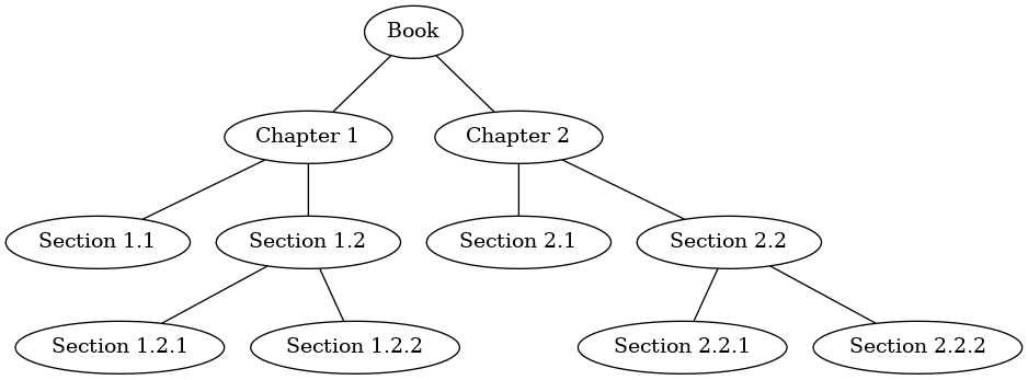
Suppose that you wanted to read this book from front to back. The preorder traversal gives you exactly that ordering.

Starting at the root of the tree (the Book node) we will follow the preorder traversal instructions. We recursively call preorder on the left child, in this case Chapter1. We again recursively call preorder on the left child to get to Section 1.1. Since Section 1.1 has no children, we do not make any additional recursive calls. When we are finished with Section 1.1, we move up the tree to Chapter 1. At this point we still need to visit the right subtree of Chapter 1, which is Section 1.2. As before we visit the left subtree, which brings us to Section 1.2.1, then we visit the node for Section 1.2.2. With Section 1.2 finished, we return to Chapter 1. Then we return to the Book node and follow the same procedure for Chapter 2.

The code for writing tree traversals is surprisingly elegant, largely because the traversals are written recursively. The code belwo shows a version of the preorder traversal written as an external function that takes a binary tree as a parameter. The external function is particularly elegant because our base case is simply to check if the tree exists. If the tree parameter is None, then the function returns without taking any action.

def preorder(tree):
    if tree:
        print(tree._key, end=" ")
        preorder(tree._left_child)
        preorder(tree._right_child)

preorder(pt)

+ 3 * 4 5 

load_anim("preorder")

前序走訪 Preorder — root → 左 → 右

›點「開始」播放動畫，或用「單步」逐步觀察

輸出將顯示在此 →

Preorder 前序 Inorder 中序 Postorder 後序

解析樹 (3+(4*5)) BST 範例 完整二元樹

▶ 開始 → 單步 ↺ 重置

速度

虛擬碼 CODE

def preorder(tree):     if tree:         print(tree._key, end=" ")         preorder(tree._left_child)         preorder(tree._right_child)

遞迴呼叫堆疊 STACK

call stack ↓

We can also implement preorder as a method of the BinaryTree class. The code for implementing preorder as an internal method. Notice what happens when we move the code from external to internal. In general, we just replace tree with self. However, we also need to modify the base case. The internal method must check for the existence of the left and the right children before making the recursive call to preorder.

def preorder(self):
    print(self.key)
    if self.left_child:
        self.left_child.preorder()
    if self.right_child:
        self.right_child.preorder()

Implementing preorder as an external function is probably better in this case. The reason is that you very rarely want to just traverse the tree. In most cases you are going to want to accomplish something else while using one of the basic traversal patterns.

In fact, we will see in the next example that the postorder traversal pattern follows very closely with the code we wrote earlier to evaluate a parse tree. Therefore we will write the rest of the traversals as external functions.

def postorder(tree):
    if tree:
        postorder(tree._left_child)
        postorder(tree._right_child)
        print(tree._key, end=" ")

postorder(pt)

3 4 5 * + 

load_anim("postorder")

後序走訪 Postorder — 左 → 右 → root

›點「開始」播放動畫,或用「單步」逐步觀察

輸出將顯示在此 →

Preorder 前序 Inorder 中序 Postorder 後序

解析樹 (3+(4*5)) BST 範例 完整二元樹

▶ 開始 → 單步 ↺ 重置

速度

虛擬碼 CODE

def postorder(tree):     if tree:         postorder(tree._left_child)         postorder(tree._right_child)         print(tree._key, end=" ")

遞迴呼叫堆疊 STACK

call stack ↓

We have already seen a common use for the postorder traversal, namely evaluating a parse tree. Assuming our binary tree is going to store only expression tree data, rewrite the evaluation function, but model it even more closely on the postorder code, we have:

def postordereval(tree):
    operators = {
        "+": operator.add,
        "-": operator.sub,
        "*": operator.mul,
        "/": operator.truediv,
    }
    result_1 = None
    result_2 = None
    if tree:
        result_1 = postordereval(tree._left_child)
        result_2 = postordereval(tree._right_child)
        if result_1 and result_2:
            return operators[tree._key](result_1, result_2)
        return tree._key

postordereval(pt)

23

Note that except that instead of printing the key at the end of the function, we return it. This allows us to save the values returned from the recursive calls. We then use these saved values along with the operator.

The final traversal we will look at in this section is the inorder traversal. In the inorder traversal we visit the left subtree, followed by the root, and finally the right subtree.

def inorder(tree):
    if tree:
        inorder(tree._left_child)
        print(tree._key, end=" ")
        inorder(tree._right_child)

inorder(pt)

3 + 4 * 5 

load_anim("inorder")

中序走訪 Inorder — 左 → root → 右

›點「開始」播放動畫，或用「單步」逐步觀察

輸出將顯示在此 →

Preorder 前序 Inorder 中序 Postorder 後序

解析樹 (3+(4*5)) BST 範例 完整二元樹

▶ 開始 → 單步 ↺ 重置

速度

虛擬碼 CODE

def inorder(tree):     if tree:         inorder(tree._left_child)         print(tree._key, end=" ")         inorder(tree._right_child)

遞迴呼叫堆疊 STACK

call stack ↓

If we perform a simple inorder traversal of a parse tree, we get our original expression back without any parentheses. Let's modify the basic inorder algorithm to allow us to recover the fully parenthesized version of the expression. The only modifications we will make to the basic template are as follows.

Print a left parenthesis before the recursive call to the left subtree, and print a right parenthesis after the recursive call to the right subtree:

def print_exp(tree):
    result = ""
    if tree:
        result = "(" + print_exp(tree._left_child)
        result = result + str(tree._key)
        result = result + print_exp(tree._right_child) + ")"
    return result

print_exp(pt)

'((3)+((4)*(5)))'

display_quiz(path+"traversal.json", max_width=800)

Exercise 1: Clean up the print_exp() function so that it does not include an extra set of parentheses around each number.

def print_exp(tree):
    result = ""
    if tree:
        result = "(" + print_exp(tree._left_child)
        result = result + str(tree._key)
        result = result + print_exp(tree._right_child) + ")"
    return result

print_exp(pt)

'((3)+((4)*(5)))'

6.9. Priority Queues with Binary Heaps

You can probably think of a couple of easy ways to implement a priority queue using sorting functions and lists. However, inserting into a list is $O(n)$ and sorting a list is $O(n \log{n})$.

We can do better. The classic way to implement a priority queue is using a data structure called a binary heap. A binary heap will allow us both to enqueue and dequeue items in $O(\log{n})$.

The binary heap is interesting to study because when we diagram the heap it looks a lot like a tree, but when we implement it we use only a single list as an internal representation. The binary heap has two common variations: the min heap, in which the smallest key value is always at the front, and the max heap, in which the largest key value is always at the front. In this section we will implement the min heap.

6.10. Binary Heap Operations

• BinaryHeap(): creates a new empty binary heap.

• insert(k): adds a new item to the heap.

• get_min(): returns the item with the minimum key value, leaving the item in the heap.

• delete(): returns the item with the minimum key value, removing the item from the heap.

• is_empty(): returns True if the heap is empty, False otherwise.

• size(): returns the number of items in the heap.

• heapify(list): builds a new heap from a list of keys.

from pythonds3.trees import BinaryHeap

my_heap = BinaryHeap()
my_heap.insert(5)
my_heap.insert(7)
my_heap.insert(3)
my_heap.insert(11)

print(my_heap.delete())
print(my_heap.delete())
print(my_heap.delete())
print(my_heap.delete())

3
5
7
11

from pythonds3.trees import BinaryHeap

my_heap = BinaryHeap()
my_heap.insert(10)
print(my_heap)
my_heap.insert(4)
print(my_heap)
my_heap.insert(9)
print(my_heap)
my_heap.insert(8)
print(my_heap)
my_heap.insert(12)
print(my_heap)
my_heap.insert(15)
print(my_heap)
my_heap.insert(3)
print(my_heap)
my_heap.insert(5)
print(my_heap)
my_heap.insert(14)
print(my_heap)
my_heap.insert(18)

print(my_heap)

[10]
[4, 10]
[4, 10, 9]
[4, 8, 9, 10]
[4, 8, 9, 10, 12]
[4, 8, 9, 10, 12, 15]
[3, 8, 4, 10, 12, 15, 9]
[3, 5, 4, 8, 12, 15, 9, 10]
[3, 5, 4, 8, 12, 15, 9, 10, 14]
[3, 5, 4, 8, 12, 15, 9, 10, 14, 18]

Notice that no matter what order we add items to the heap, the smallest is removed each time!

6.11. Binary Heap Implementation

In order to make our heap work efficiently, we will take advantage of the logarithmic nature of the binary tree to represent our heap.

In order to guarantee logarithmic performance, we must keep our tree balanced. A balanced binary tree has roughly the same number of nodes in the left and right subtrees of the root. In our heap implementation we keep the tree balanced by creating a complete binary tree.

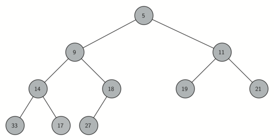
A complete binary tree is a tree in which each level has all of its nodes. The exception to this is the bottom level of the tree, which we fill in from left to right. Figure below shows an example of a complete binary tree.

Another interesting property of a complete tree is that we can represent it using a single list. We do not need to use nodes and references or even lists of lists. Because the tree is complete, the left child of a parent (at position $p$) is the node that is found in position $2p+1$ in the list!

Similarly, the right child of the parent is at position $2p+2$ in the list. To find the parent of any node in the tree, we can simply use integer division. Given that a node is at position $n$ in the list, the parent is at position $(n - 1) // 2$.

Figure below shows a complete binary tree and also gives the list representation of the tree. Note the $2p+1$ and $2p+2$ relationship between parent and children.

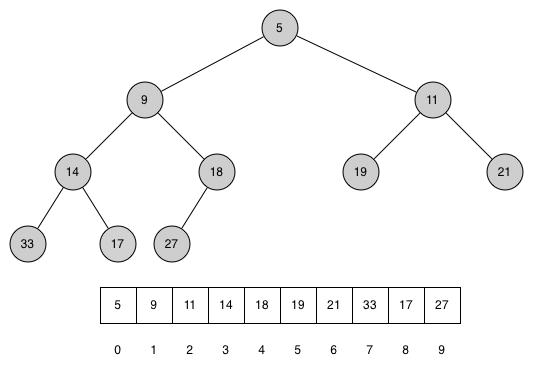
The list representation of the tree, along with the full structure property, allows us to efficiently traverse a complete binary tree using only a few simple mathematical operations.

The method that we will use to store items in a heap relies on maintaining the heap order property. The heap order property is as follows: in a heap, for every node $x$ with parent $p$, the key in $p$ is smaller than or equal to the key in $x$. Figure above also illustrates a complete binary tree that has the heap order property.

We now begin our implementation of a binary heap with the constructor. Since the entire binary heap can be represented by a single list, all the constructor will do is initialize the list:

class BinaryHeap:
    def __init__(self):
        self._heap = []

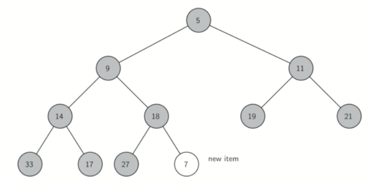
The next method we will implement is insert(). The easiest, and most efficient, way to add an item to a list is to simply append the item to the end of the list. The good news about appending is that it guarantees that we will maintain the complete tree property. The bad news about appending is that we will very likely violate the heap structure property.

However, it is possible to write a method that will allow us to regain the heap structure property by comparing the newly added item with its parent. If the newly added item is less than its parent, then we can swap the item with its parent.

Figure below shows the series of swaps needed to percolate the newly added item up to its proper position in the tree.

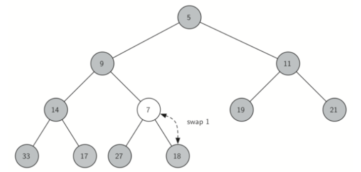
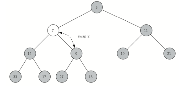
Notice that when we percolate an item up, we are restoring the heap property between the newly added item and the parent. We are also preserving the heap property for any siblings. Of course, if the newly added item is very small, we may still need to swap it up another level. In fact, we may need to keep swapping until we get to the top of the tree!

def _perc_up(self, i):
    while (i - 1) // 2 >= 0:
        parent_idx = (i - 1) // 2
        if self._heap[i] < self._heap[parent_idx]:
            self._heap[i], self._heap[parent_idx] = (
                self._heap[parent_idx],
                self._heap[i],
            )
        i = parent_idx

We are now ready to write the insert() method. Most of the work in the insert() method is really done by _perc_up(). Once a new item is appended to the tree, _perc_up() takes over and positions the new item properly.

load_anim("heap_insert")

Min-Heap Insert — perc_up 動畫

陣列表示（heap[i]）：

›輸入 key 後按「插入」或「開始」

Insert Delete-min Heapify (建堆積)

插入 key： 插入 當前 heap： 套用

▶ 開始 → 單步 ↺ 重置

速度

虛擬碼 CODE

def _perc_up(self, i):     while (i - 1) // 2 >= 0:         p = (i - 1) // 2         if heap[i] < heap[p]:             swap(heap[i], heap[p])         i = p

def insert(self, item):
    self._heap.append(item)
    self._perc_up(len(self._heap) - 1)

With the insert() method properly defined, we can now look at the delete() method. Since the heap property requires that the root of the tree be the smallest item in the tree, finding the minimum item is easy.

The hard part of delete is restoring full compliance with the heap structure and heap order properties after the root has been removed. We can restore our heap in two steps.

First, we will restore the root item by taking the last item in the list and moving it to the root position. Moving the last item maintains our heap structure property. However, we have probably destroyed the heap order property of our binary heap.

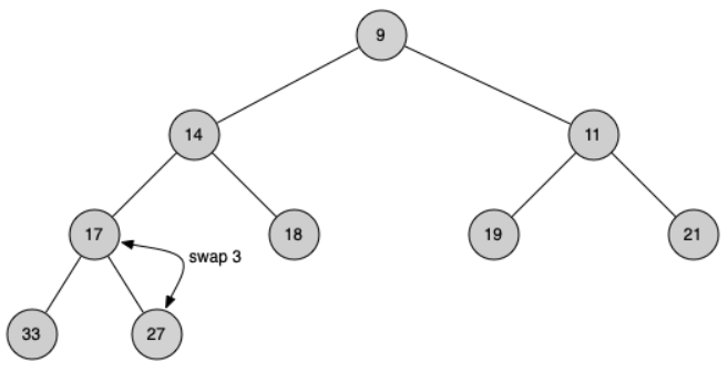
Second, we will restore the heap order property by pushing the new root node down the tree to its proper position. Figure below shows the series of swaps needed to move the new root node to its proper position in the heap.

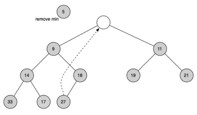
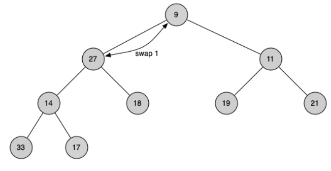
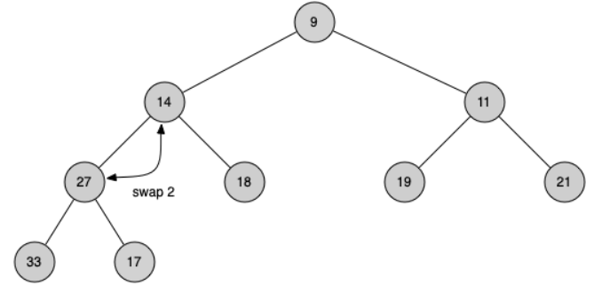
In order to maintain the heap order property, all we need to do is swap the root with its smaller child that is less than the root. After the initial swap, we may repeat the swapping process with a node and its children until the node is swapped into a position on the tree where it is already less than both children.

def _perc_down(self, i):
    while 2 * i + 1 < len(self._heap):
        sm_child = self._get_min_child(i)
        if self._heap[i] > self._heap[sm_child]:
            self._heap[i], self._heap[sm_child] = (
                self._heap[sm_child],
                self._heap[i],
            )
        else:
            break
        i = sm_child

def _get_min_child(self, i):
    if 2 * i + 2 > len(self._heap) - 1:
        return 2 * i + 1
    if self._heap[2 * i + 1] < self._heap[2 * i + 2]:
        return 2 * i + 1
    return 2 * i + 2

The code for the delete operation is in below. Note that once again the hard work is handled by a helper function, in this case _perc_down().

def delete(self):
    self._heap[0], self._heap[-1] = self._heap[-1], self._heap[0]
    result = self._heap.pop()
    self._perc_down(0)
    return result

load_anim("heap_extract")

Min-Heap Delete-min — perc_down 動畫

陣列表示（heap[i]）：

›按「開始」執行 delete-min

Insert Delete-min Heapify (建堆積)

插入 key： 插入 當前 heap： 套用

▶ 開始 → 單步 ↺ 重置

速度

虛擬碼 CODE

def delete_min(self):     m = heap[0]     heap[0] = heap.pop()     self._perc_down(0)     return m

To finish our discussion of binary heaps, we will look at a method to build an entire heap from a list of keys. The first method you might think of may be like the following. Given a list of keys, you could easily build a heap by inserting each key one at a time. Since you are starting with an empy list, it is sorted and you could use binary search to find the right position to insert the next key at a cost of approximately $O(\log{n})$ operations.

However, remember that inserting an item in the middle of the list may require $O(n)$ operations to shift the rest of the list over to make room for the new key.

Therefore, to insert $n$ keys into the heap would require a total of $O(n^2)$ operations. However, if we start with an entire list then we can build the whole heap in $O(n)$ operations.

def heapify(self, not_a_heap):
    self._heap = not_a_heap[:]
    i = len(self._heap) // 2 - 1
    while i >= 0:
        self._perc_down(i)
        i = i - 1

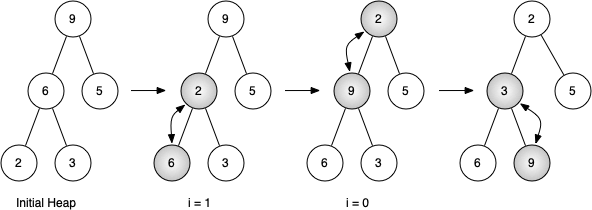
Figure above shows the swaps that the hepify() method makes as it moves the nodes in an initial tree of [9, 6, 5, 2, 3] into their proper positions. Although we start out in the middle of the tree and work our way back toward the root, the _perc_down() method ensures that the largest child is always moved down the tree. Because the heap is a complete binary tree, any nodes past the halfway point will be leaves and therefore have no children!

Notice that when i = 0, we are percolating down from the root of the tree, so this may require multiple swaps. As you can see in the rightmost two trees of the figure, first the 9 is moved out of the root position, but after 9 is moved down one level in the tree, _perc_down() ensures that we check the next set of children farther down in the tree to ensure that it is pushed as low as it can go.

In this case it results in a second swap with 3. Now that 9 has been moved to the lowest level of the tree, no further swapping can be done.

load_anim("heap_build")

Heapify — 從未排序陣列建堆積（O(n)）

陣列表示（heap[i]）：

›陣列當作未排序輸入,按「開始」做 heapify

Insert Delete-min Heapify (建堆積)

插入 key： 插入 當前 heap： 套用

▶ 開始 → 單步 ↺ 重置

速度

虛擬碼 CODE

def build_heap(self, arr):     self.heap = arr     i = len(arr) // 2 - 1     while i >= 0:         self._perc_down(i)         i -= 1

為什麼是 O(n)？

底層大量節點高度只有 0/1，移動成本極小；頂層節點少但移動多。總和 $\sum \frac{n}{2^{h+1}} \cdot h = O(n)$。

start  [9, 6, 5, 2, 3]
i = 1  [9, 2, 5, 6, 3]
i = 0  [2, 3, 5, 6, 9]

import sys
sys.path.append("./pythonds3/")
from pythonds3.trees import BinaryHeap

a_heap = BinaryHeap()
a_heap.heapify([10, 4, 9, 8, 12, 15, 3, 5, 14, 18])

#while not a_heap.is_empty():
#    print(a_heap.delete())
print(a_heap)

[3, 4, 9, 5, 12, 15, 10, 8, 14, 18]

The assertion that we can build the heap in $O(n)$ may seem a bit mysterious at first, and a proof is beyond the scope of this course. However, the key to understanding that you can build the heap in $O(n)$ is to remember that the $\log{n}$ factor is derived from the height of the tree. For most of the work in heapify(), the tree is shorter than $\log{n}$.

display_quiz(path+"binary_heap.json", max_width=800)

Using the fact that you can build a heap from a list in $O(n)$ time, you will construct a sorting algorithm that uses a heap and sorts a list in $O(n\log{n})$ as an exercise at the end of this chapter.

https://visualgo.net/en/heap

Exercise 2: Using the heapify() and delete() method, write a sorting function that can sort a list in $O(n\log n)$ time.

def heap_sort(unsorted_list) :
    """Sorts a list using heap sort."""
    heap = BinaryHeap()
    # 1. Build the heap in O(n) time

    # 2. The main sorting loop involves calling delete on the heap 
    # to get the smallest element and adding this to the sorted list.
    # Each delete operation is O(log n)

# Example list to be sorted
unsorted_list = [10, 3, 5, 1, 15, 7, 9, 2, 8]

# Sort the list using heap sort
sorted_list = heap_sort(unsorted_list)

# Print the sorted list
print("Sorted list:", sorted_list)

Sorted list: None

6.12. Binary Search Trees

We have already seen two different ways to get key-value pairs in a collection. Recall that these collections implement the map abstract data type. The two implementations of the map ADT that we have discussed were binary search on a list and hash tables.

In this section we will study binary search trees as yet another way to map from a key to a value. In this case we are not interested in the exact placement of items in the tree, but we are interested in using the binary tree structure to provide for efficient searching.

6.13. Search Tree Operations

Before we look at the implementation, let's review the interface provided by the map ADT. You will notice that this interface is very similar to the dictionary.

• Map(): creates a new empty map.

• put(key, val): adds a new key–value pair to the map. If the key is already in the map, it replaces the old value with the new value.

• get(key): takes a key and returns the matching value stored in the map or None otherwise.

• del: deletes the key–value pair from the map using a statement of the form del map[key].

• size(): returns the number of key–value pairs stored in the map.

• in: return True for a statement of the form key in map if the given key is in the map, False otherwise.

6.14. Search Tree Implementation

A binary search tree (BST) relies on the property that keys that are less than the parent are found in the left subtree, and keys that are greater than the parent are found in the right subtree. We will call this the BST property.

Figure below illustrates this property of a binary search tree, showing the keys without any associated values.

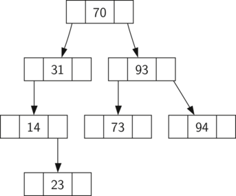
Notice that the property holds for each parent and child. All of the keys in the left subtree are less than the key in the root. All of the keys in the right subtree are greater than the root.

Now that you know what a binary search tree is, we will look at how a binary search tree is constructed. The search tree above represents the nodes that exist after we have inserted the following keys in the order shown: $70, 31, 93, 94, 14, 23, 73$. Since 70 was the first key inserted into the tree, it is the root.

Next, 31 is less than 70, so it becomes the left child of 70. Next, 93 is greater than 70, so it becomes the right child of 70. Now we have two levels of the tree filled, so the next key is going to be the left or right child of either 31 or 93.

Since 94 is greater than 70 and 93, it becomes the right child of 93. Similarly 14 is less than 70 and 31, so it becomes the left child of 31. 23 is also less than 31, so it must be in the left subtree of 31. However, it is greater than 14, so it becomes the right child of 14.

load_anim("bst_search")

BST 搜尋 (get) — 沿樹下移比較 key

›輸入 key 後按 get 進行搜尋

初始 keys： 建立樹 隨機

搜尋 key： put (插入) get (搜尋)

→ 單步 ↺ 重置

速度

虛擬碼 — _get CODE

def _get(self, key, current_node):     if not current_node: return None     if current_node.key == key:         return current_node     elif key < current_node.key:         return self._get(key, current_node.left_child)     else:         return self._get(key, current_node.right_child)

To implement the binary search tree, we will use the nodes and references approach similar to the one we used to implement the linked list and the expression tree.

However, because we must be able create and work with a binary search tree that is empty, our implementation will use two classes. The first class we will call BinarySearchTree, and the second class we will call TreeNode.

The BinarySearchTree class has a reference to the TreeNode that is the root of the binary search tree. In most cases the external methods defined in the outer class simply check to see if the tree is empty. If there are nodes in the tree, the request is just passed on to a private method defined in the BinarySearchTree class that takes the root as a parameter.

In the case where the tree is empty or we want to delete the key at the root of the tree, we must take special action.

class BinarySearchTree:
    def __init__(self):
        self.root = None
        self.size = 0

    def __len__(self):
        return self.size

    def __iter__(self):
        return self.root.__iter__()

The TreeNode class provides many helper methods that make the work done in the BinarySearchTree class methods much easier.

Many of these helper methods help to classify a node according to its own position as a child (left or right) and the kind of children the node has.

class TreeNode:
    def __init__(self, key, value, left=None, right=None, parent=None):
        self.key = key
        self.value = value
        self.left_child = left
        self.right_child = right
        self.parent = parent

    def is_left_child(self):
        return self.parent and self.parent.left_child is self
    def is_right_child(self):
        return self.parent and self.parent.right_child is self
    def is_root(self):
        return not self.parent
    def is_leaf(self):
        return not (self.right_child or self.left_child)
    def has_any_child(self):
        return self.right_child or self.left_child
    def has_children(self):
        return self.right_child and self.left_child

    def replace_value(self, key, value, left, right):
        self.key = key
        self.value = value
        self.left_child = left
        self.right_child = right
        if self.left_child:
            self.left_child.parent = self
        if self.right_child:
            self.right_child.parent = self

The TreeNode class will also explicitly keep track of the parent as an attribute of each node. You will see why this is important when we discuss the implementation for the del operator.

Another interesting aspect is that we use optional parameters which make it easy for us to create a TreeNode under several different circumstances.

Sometimes we will want to construct a new TreeNode that already has both a parent and a child (e.g. left) and in that case we can pass parent and left_child as parameters.

At other times we will just create a TreeNode with the key-value pair, and we will not pass any parameters for parent or child. In this case, the default values of the optional parameters are used.

Now that we have the BinarySearchTree shell and the TreeNode, it is time to write the put() method that will allow us to build our binary search tree. The method is a method of the BinarySearchTree class. This method will check to see if the tree already has a root. If there is not a root, then put() will create a new TreeNode and install it as the root of the tree.

If a root node is already in place, then put() calls the private recursive helper method _put() to search the tree according to the following algorithm.

• Starting at the root of the tree, search the binary tree comparing the new key to the key in the current node. If the new key is less than the current node, search the left subtree. If the new key is greater than the current node, search the right subtree.

• When there is no left or right child to search, we have found the position in the tree where the new node should be installed.

• To add a node to the tree, create a new TreeNode object and insert the object at the point discovered in the previous step.

def put(self, key, value):
    if self.root:
        self._put(key, value, self.root)
    else:
        self.root = TreeNode(key, value)
    self.size = self.size + 1

def _put(self, key, value, current_node):
    if key < current_node.key:
        if current_node.left_child:
            self._put(key, value, current_node.left_child)
        else:
            current_node.left_child = TreeNode(key, value, 
                                               parent=current_node)
    else:
        if current_node.right_child:
            self._put(key, value, current_node.right_child)
        else:
            current_node.right_child = TreeNode(key, value, 
                                                parent=current_node)

Notice that when a new child is inserted into the tree, the current_node is passed to the new tree as the parent.

One important problem with our implementation of insertion is that duplicate keys are not handled properly. A duplicate key will create a new node with the same key value in the right subtree of the node having the original key. The result of this is that the node with the new key will never be found during a search!

A better way to handle the insertion of a duplicate key is for the value associated with the new key to replace the old value. We leave fixing this bug as an exercise for you.

With the put() method defined, we can easily overload the [] operator for assignment. This allows us to write statements like my_zip_tree['Plymouth'] = 55446, just like a Python dictionary!

def __setitem__(self, key, value):
    self.put(key, value)

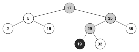
Figure below illustrates the process for inserting a new node into a binary search tree. The lightly shaded nodes indicate the nodes that were visited during the insertion process.

load_anim("bst_insert")

BST 插入 (put) — 沿 BST 性質找空位

›輸入 key 後按 put 進行插入

初始 keys： 建立樹 隨機

插入 key： put (插入) get (搜尋)

→ 單步 ↺ 重置

速度

虛擬碼 — _put CODE

def _put(self, key, value, current_node):     if key < current_node.key:         if current_node.left_child:             self._put(key, value, current_node.left_child)         else:             current_node.left_child = TreeNode(key, value, parent=current_node)     else:         if current_node.right_child:             self._put(key, value, current_node.right_child)         else:             current_node.right_child = TreeNode(key, value, parent=current_node)

The get() method is even easier than the put() method because it simply searches the tree recursively until it gets to a non-matching leaf node or finds a matching key. When a matching key is found, the value stored in the payload of the node is returned.

def get(self, key):
    if self.root:
        result = self._get(key, self.root)
        if result:
            return result.value
    return None

def _get(self, key, current_node):
    if not current_node:
        return None
    if current_node.key == key:
        return current_node
    elif key < current_node.key:
        return self._get(key, current_node.left_child)
    else:
        return self._get(key, current_node.right_child)

Notice that the _get() method returns a TreeNode to get(), this allows _get() to be used as a flexible helper method for other BinarySearchTree methods that may need to make use of other data from the TreeNode besides the payload!

We can implement two to related methods as follows:

def __getitem__(self, key):
    return self.get(key)

def __contains__(self, key):
    return bool(self._get(key, self.root))

Finally, we turn our attention to the most challenging operation on the binary search tree, the deletion of a key. The first task is to find the node to delete by searching the tree. If the tree has more than one node we search using the _get() method to find the TreeNode that needs to be removed.

If the tree only has a single node, that means we are removing the root of the tree, but we still must check to make sure the key of the root matches the key that is to be deleted!

def delete(self, key):
    if self.size > 1:
        node_to_remove = self._get(key, self.root)
        if node_to_remove:
            self._delete(node_to_remove)
            self.size = self.size - 1
        else:
            raise KeyError("Error, key not in tree")
    elif self.size == 1 and self.root.key == key:
        self.root = None
        self.size = self.size - 1
    else:
        raise KeyError("Error, key not in tree")

Once we've found the node containing the key we want to delete, there are three cases that we must consider:

1. The node to be deleted has no children

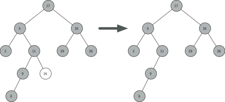
The first case is straightforward. If the current node has no children, all we need to do is delete the node and remove the reference to this node in the parent.

if current_node.is_leaf():
    if current_node == current_node.parent.left_child:
        current_node.parent.left_child = None
    else:
        current_node.parent.right_child = None

2. The node to be deleted has only one child

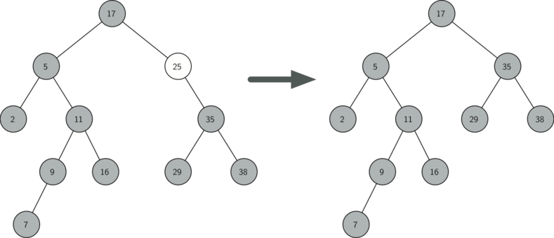
The second case is only slightly more complicated. If a node has only a single child, then we can simply promote the child to take the place of its parent. Since the cases are symmetric with respect to either having a left or right child, we will just discuss the case where the current node has a left child.

1. If the current node is a left child, then we only need to update the parent reference of the left child to point to the parent of the current node, and then update the left child reference of the parent to point to the current node's left child.

2. If the current node is a right child, then we only need to update the parent reference of the left child to point to the parent of the current node, and then update the right child reference of the parent to point to the current node’s left child.

3. If the current node has no parent, it must be the root. In this case we will just replace the key, value, left_child, and right_child data by calling the replace_value() method on the root.

else:  # removing a node with one child
    if current_node.get_left_child():
        if current_node.is_left_child():
            current_node.left_child.parent = current_node.parent
            current_node.parent.left_child = current_node.left_child
        elif current_node.is_right_child():
            current_node.left_child.parent = current_node.parent
            current_node.parent.right_child = current_node.left_child
        else:
            current_node.replace_value(
                current_node.left_child.key,
                current_node.left_child.value,
                current_node.left_child.left_child,
                current_node.left_child.right_child,
            )
    else:    
        

3. The node to be deleted has two children

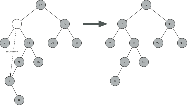
The third case is the most difficult case to handle. If a node has two children, then it is unlikely that we can simply promote one of them to take the node's place!

We can, however, search the tree for a node that can be used to replace the one scheduled for deletion. What we need is a node that will preserve the bst relationships for both of the existing left and right subtrees. The node that will do this is the node that has the next-largest key in the tree. We call this node the successor.

The successor is guaranteed to have no more than one child, so we know how to remove it using the two cases for deletion that we have already implemented. Once the successor has been removed, we simply put it in the tree in place of the node to be deleted. We make use of the helper methods find_successor() and splice_out() to find and remove the successor. The reason we use splice_out() is that it goes directly to the node we want to splice out and makes the right changes.

elif current_node.has_children():  # removing a node with two children
    successor = current_node.find_successor()
    successor.splice_out()
    current_node.key = successor.key
    current_node.value = successor.value

def find_successor(self): # a method of the TreeNode class
    successor = None
    if self.right_child:
        successor = self.right_child.find_min()
    else:
        if self.parent:
            if self.is_left_child():
                successor = self.parent
            else:
                self.parent.right_child = None
                successor = self.parent.find_successor()
                self.parent.right_child = self
    return successor

def find_successor(self): # a method of the TreeNode class
    successor = None
    successor = self.right_child.find_min()
    return successor

This code makes use of the same properties of binary search trees that cause an inorder traversal to print out the nodes in the tree from smallest to largest. In general, there are three cases to consider when looking for the successor:

1. If the node has a right child, then the successor is the smallest key in the right subtree.

2. If the node has no right child and is the left child of its parent, then the parent is the successor.

3. If the node is the right child of its parent, and itself has no right child, then the successor to this node is the successor of its parent, excluding this node.

But here we only care about the first one since we have children!

The first condition is the only one that matters for us when deleting a node from a binary search tree. However, the find_successor method has other uses that we will explore in the exercises at the end of this chapter.

def find_min(self):
    current = self
    while current.left_child:
        current = current.left_child
    return current

The find_min() method is called to find the minimum key in a subtree. You should convince yourself that the minimum value key in any binary search tree is the leftmost child of the tree. Therefore the find_min() method simply follows the left_child references in each node of the subtree until it reaches a node that does not have a left child.

def splice_out(self):
    if self.is_leaf():
        if self.is_left_child():
            self.parent.left_child = None
        else:
            self.parent.right_child = None
    elif self.has_any_child():
        if self.left_child:
            if self.is_left_child():
                self.parent.left_child = self.left_child
            else:
                self.parent.right_child = self.left_child
            self.left_child.parent = self.parent
        else:
            if self.is_left_child():
                self.parent.left_child = self.right_child
            else:
                self.parent.right_child = self.right_child
            self.right_child.parent = self.parent

load_anim("bst_delete")

BST 刪除 — 三種情境與 in-order successor

›點選下方 case 預設或輸入 key 後按「刪除」

樹結構（依序插入）： 建立樹

刪除 key： ▶ 刪除 → 單步 ↺ 重建

Case 1：刪 20（葉） Case 2：刪 80（一子） Case 3：刪 30（兩子） Case 3：刪 50（root）

當前情境 CASE

情境—

target key—

successor—

階段—

find_successor CODE

def find_successor(self):     if self.right_child:         return self.right_child.find_min()     ... def find_min(self):     cur = self     while cur.left_child:         cur = cur.left_child     return cur

We need to look at one last interface method for the binary search tree. Suppose that we would like to simply iterate over all the keys in the tree in order. You already know how to traverse a binary tree in order, using the inorder traversal algorithm. However, writing an iterator requires a bit more work since an iterator should return only one node each time the iterator is called.

def __iter__(self):
    if self:
        if self.left_child:
            for elem in self.left_child:
                yield elem
        yield self.key
        if self.right_child:
            for elem in self.right_child:
                yield elem

yield is similar to return in that it returns a value to the caller. However, yield also takes the additional step of freezing the state of the function so that the next time the function is called it continues executing from the exact point it left off earlier. Functions that create objects that can be iterated are called generator functions.

At first glance you might think that the code is not recursive. However, remember that __iter__ overrides the for ... in operation for iteration, so it really is recursive!

import sys
sys.path.append("./pythonds3/")

from pythonds3.trees import BinarySearchTree

my_tree = BinarySearchTree()
my_tree["a"], my_tree["q"] = "a", "quick"
my_tree["b"], my_tree["f"] = "brown", "fox"
my_tree["j"], my_tree["o"] = "jumps", "over"
my_tree["t"], my_tree["l"] = "the", "lazy"
my_tree["d"] = "dog"

print(my_tree["q"])
print(my_tree["l"])
print("There are {} items in this tree".format(len(my_tree)))
my_tree.delete("a")
print("There are {} items in this tree".format(len(my_tree)))

for node in my_tree:
    print(my_tree[node], end=" ")
print()

quick
lazy
There are 9 items in this tree
There are 8 items in this tree
brown dog fox jumps lazy over quick the 

https://visualgo.net/en/bst

Exercise 3: Using the put() and in method, write a sorting function that can sort a list in $O(n\log n)$ time in average case.

def tree_sort(values):
    bst = BinarySearchTree()
    # 1. Insert all elements into the BST. Each insert is O(log n) on average,
    # leading to O(n log n) for all insertions if the tree is balanced.

    # 2. Perform an in-order traversal of the BST. This operation is O(n)
    # because each node is visited exactly once in sorted order.

# Example list to be sorted
unsorted_list = [20, 1, 15, 22, 10, 3, 7, 5, 8, 12]

# Sort the list using tree sort
sorted_list = tree_sort(unsorted_list)

# Print the sorted list
print("Sorted list:", sorted_list)

Sorted list: None

6.15. Search Tree Analysis

Let's first look at the put() method. The limiting factor on its performance is the height of the binary tree. Recall from the vocabulary section that the height of a tree is the number of edges between the root and the deepest leaf node.

The height is the limiting factor because when we are searching for the appropriate place to insert a node into the tree, we will need to do at most one comparison at each level of the tree!

Note that if the keys are added in a random order, the height of the tree is going to be around $\log_2{n}$ where $n$ is the number of nodes in the tree. This is because if the keys are randomly distributed, about half of them will be less than the root and about half will be greater than the root.

Remember that in a binary tree there is one node at the root, two nodes in the next level, and four at the next. The number of nodes at any particular level is $2^d$ where $d$ is the depth of the level. The total number of nodes in a perfectly balanced binary tree is $2^{h+1}-1$, where $h$ represents the height of the tree.

A perfectly balanced tree has the same number of nodes in the left subtree as the right subtree. In a balanced binary tree, the worst-case performance of put() is $O(\log_2{n})$.

Notice that this is the inverse relationship to the calculation in the previous paragraph. So $\log_2{n}$ gives us the height of the tree and represents the maximum number of comparisons that put() will need to do as it searches for the proper place to insert a new node.

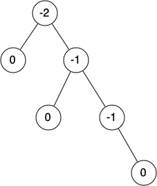
Unfortunately it is possible to construct a search tree that has height $n$ simply by inserting the keys in sorted order! An example of this is shown below:

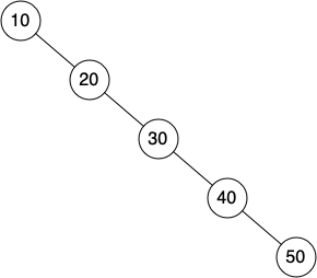
In this case the performance of the put method is $O(n)$.

Now that you understand that the performance of the put() method is limited by the height of the tree, you can probably guess that other methods, get(), in, and del, are limited as well. Since get() searches the tree to find the key, in the worst case the tree is searched all the way to the bottom and no key is found.

At first glance del might seem more complicated since it may need to search for the successor before the deletion operation can complete. But remember that the worst-case scenario to find the successor is also just the height of the tree which means that you would simply double the work. Since doubling is a constant factor, it does not change worst-case analysis of $O(n)$ for an unbalanced tree.

display_quiz(path+"bst.json", max_width=800)

6.16. Balanced Binary Search Trees

In the previous section we looked at building a binary search tree. As we learned, the performance of the binary search tree can degrade to $O(n)$ for operations like get() and put() when the tree becomes unbalanced.

In this section we will look at a special kind of binary search tree that automatically makes sure that the tree remains balanced at all times. This tree is called an AVL tree.

An AVL tree implements the Map abstract data type just like a regular binary search tree; the only difference is in how the tree performs. To implement our AVL tree we need to keep track of a balance factor for each node in the tree.

We do this by looking at the heights of the left and right subtrees for each node. More formally, we define the balance factor for a node as the difference between the height of the left subtree and the height of the right subtree.

$$balance\_factor = height(left\_subtree) - height(right\_subtree)$$

Using the definition for balance factor given above, we say that a subtree is left-heavy if the balance factor is greater than zero. If the balance factor is less than zero, then the subtree is right-heavy. If the balance factor is zero, then the tree is perfectly in balance.

For purposes of implementing an AVL tree and gaining the benefit of having a balanced tree, we will define a tree to be in balance if the balance factor is -1, 0, or 1. Once the balance factor of a node in a tree is outside this range we will need to have a procedure to bring the tree back into balance.

Below shows an example of an unbalanced right-heavy tree and the balance factors of each node:

6.17. AVL Tree Performance (Optional)

Before we proceed any further let's look at the result of enforcing this new balance factor requirement. Our claim is that by ensuring that a tree always has a balance factor of -1, 0, or 1 we can get better Big-O performance of key operations.

Let us start by thinking about how this balance condition changes the worst-case tree. There are two possibilities to consider, a left-heavy tree and a right-heavy tree. If we consider trees of heights 0, 1, 2, and 3, Figure below illustrates the most unbalanced left-heavy tree possible under the new rules.

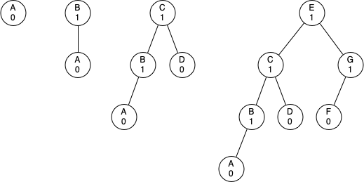
Looking at the total number of nodes in the tree we see that for a tree of height 0 there is 1 node, for a tree of height 1 there is $1 + 1 = 2$ nodes, for a tree of height 2 there are $1 + 1 + 2 = 4$, and for a tree of height 3 there are $1 + 2 + 4 = 7$. More generally the pattern we see for the number of nodes in a tree of height $N_h$ is:

$$N_h = 1 + N_{h-1} + N_{h-2}$$

This recurrence may look familiar to you because it is very similar to the Fibonacci sequence. We can use this fact to derive a formula for the height of an AVL tree given the number of nodes in the tree.

Recall that for the Fibonacci sequence the $i^{th}$ Fibonacci number is given by:

$$\begin{split}F_0 & = 0 \\ F_1 & = 1 \\ F_i & = F_{i-1} + F_{i-2} \text{ for all } i \ge 2\end{split}$$

An important mathematical result is that as the numbers of the Fibonacci sequence get larger and larger the ratio of $F_i / F_{i-1}$ becomes closer and closer to approximating the golden ratio $\Phi$ which is defined as $\Phi = \frac{1 + \sqrt{5}}{2}$.

We will simply use this equation to approximate $F_i$ as $F_i \approx \Phi^i/\sqrt{5}$. If we make use of this approximation we can rewrite the equation for $N_h$ as:

$$N_h = F_{h+3} - 1, h \ge 1$$

By replacing the Fibonacci reference with its golden ratio approximation we get:

$$N_h = \frac{\Phi^{h+2}}{\sqrt{5}} - 1$$

If we rearrange the terms, take the base 2 log of both sides, and then solve for $h$, we get the following derivation:

$$\begin{split}\log{(N_h+1)} & = (h+2)\log{\Phi} - \frac{1}{2} \log{5} \\ h & = \frac{\log{(N_h+1)} - 2 \log{\Phi} + \frac{1}{2} \log{5}}{\log{\Phi}} \\ h & \approx 1.44 \log{N_h}\end{split}$$ for large $N_h$

This derivation shows us that at any time the height of our AVL tree is equal to a constant (1.44) times the log of the number of nodes in the tree. This is great news for searching our AVL tree because it limits the search to $O(\log{n})$.

6.18. AVL Tree Implementation (Optional)

Let's look at how we will augment the procedure to insert a new key into the tree. Since all new keys are inserted into the tree as leaf nodes and we know that the balance factor for a new leaf is zero, there are no new requirements for the node that has just been inserted.

But once the new leaf is added, we must update the balance factor of its parent. How this new leaf affects the parent's balance factor depends on whether the leaf node is a left child or a right child.

If the new node is a right child, the balance factor of the parent will be reduced by one. If the new node is a left child, then the balance factor of the parent will be increased by one. This rule can be applied recursively to the grandparent of the new node, and possibly to every ancestor, all the way up to the root of the tree!

Since this is a recursive procedure, let's examine the two base cases for updating balance factors:

• The recursive call has reached the root of the tree.

• The balance factor of the parent has been adjusted to zero. You should convince yourself that once a subtree has a balance factor of zero, then the balance of its ancestor nodes does not change.

We will implement the AVL tree as a subclass of BinarySearchTree. To begin, we will override the _put() method and write a new update_balance() helper method.

def _put(self, key, value, current_node):
    if key < current_node.key:
        if current_node.left_child:
            self._put(key, value, current_node.left_child)
        else:
            current_node.left_child = AVLTreeNode(
                key, value, 0, parent=current_node
            )
            self.update_balance(current_node.left_child)
    else:
        if current_node.right_child:
            self._put(key, value, current_node.right_child)
        else:
            current_node.right_child = AVLTreeNode(
                key, value, 0, parent=current_node
            )
            self.update_balance(current_node.right_child)

def update_balance(self, node):
    if node.balance_factor > 1 or node.balance_factor < -1:
        self.rebalance(node)
        return
    if node.parent:
        if node.is_left_child():
            node.parent.balance_factor += 1
        elif node.is_right_child():
            node.parent.balance_factor -= 1

        if node.parent.balance_factor != 0:
            self.update_balance(node.parent)

This implements the recursive procedure we just described. It first checks to see if the current node is out of balance enough to require rebalancing.

If that is the case then the rebalancing is done and no further updating to parents is required. If the current node does not require rebalancing then the balance factor of the parent is adjusted. If the balance factor of the parent is nonzero then the algorithm continues to work its way up the tree toward the root by recursively calling update_balance() on the parent.

When a rebalancing of the tree is necessary, how do we do it? Efficient rebalancing is the key to making the AVL Tree work well without sacrificing performance. In order to bring an AVL Tree back into balance, we will perform one or more rotations on the tree.

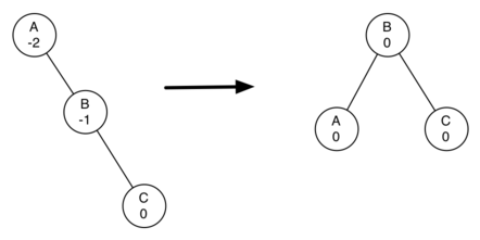
Note the tree is out of balance with a balance factor of -2. To bring this tree into balance we will use a left rotation around the subtree rooted at node A.

To perform a left rotation we essentially do the following:

1. Promote the right child (B) to be the root of the subtree.

2. Move the old root (A) to be the left child of the new root.

3. If new root (B) already has a left child, then make it the right child of the new left child (A). Note: since the new root (B) was the right child of A, the right child of A is guaranteed to be empty at this point. This allows us to add a new node as the right child without any further consideration.

While this procedure is fairly easy in concept, the details of the code are a bit tricky since we need to move things around in just the right order so that all properties of a binary search tree are preserved. Furthermore, we need to make sure to update all of the parent pointers appropriately.

Let's look at a slightly more complicated tree to illustrate the right rotation where the left side of shows a tree that is left-heavy and with a balance factor of 2 at the root:

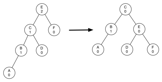
To perform a right rotation we essentially do the following:

1. Promote the left child (C) to be the root of the subtree.

2. Move the old root (E) to be the right child of the new root.

3. If the new root (C) already has a right child (D) then make it the left child of the new right child (E). Note: since the new root (C) was the left child of E, the left child of E is guaranteed to be empty at this point. This allows us to add a new node as the left child without any further consideration.

def rotate_left(self, rotation_root):
    new_root = rotation_root.right_child
    rotation_root.right_child = new_root.left_child
    if new_root.left_child:
        new_root.left_child.parent = rotation_root
    new_root.parent = rotation_root.parent
    if rotation_root.is_root():
        self._root = new_root
    else:
        if rotation_root.is_left_child():
            rotation_root.parent.left_child = new_root
        else:
            rotation_root.parent.right_child = new_root
    new_root.left_child = rotation_root
    rotation_root.parent = new_root
    rotation_root.balance_factor = (
        rotation_root.balance_factor + 1 - min(new_root.balance_factor, 0)
    )
    new_root.balance_factor = (
        new_root.balance_factor + 1 + max(rotation_root.balance_factor, 0)
    )

The code is for the left rotation (the rotate_right() method is symmetrical).

We create a temporary variable to keep track of the new root of the subtree. As we said before, the new root is the right child of the previous root. Now that a reference to the right child has been stored in this temporary variable, we replace the right child of the old root with the left child of the new.

The next step is to adjust the parent pointers of the two nodes. If new_root has a left child then the new parent of the left child becomes the old root. The parent of the new root is set to the parent of the old root. If the old root was the root of the entire tree then we must set the root of the tree to point to this new root.

Otherwise, if the old root is a left child then we change the parent of the left child to point to the new root; otherwise we change the parent of the right child to point to the new root. Finally we set the parent of the old root to be the new root.

Finally, the bottome parts require some explanation. In these lines we update the balance factors of the old and the new root. Since all the other moves involve moving entire subtrees, the balance factors of all other nodes are unaffected by the rotation.

But how can we update the balance factors without completely recalculating the heights of the new subtrees? Figure below and the following derivation should convince you that these lines are correct.

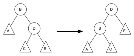
Figure above shows a left rotation. B and D are the pivotal nodes and A, C, E are their subtrees. Let $h_x$ denote the height of a particular subtree rooted at node $x$. By definition we know the following:

$$\begin{split}new\_bal(B) = h_A - h_C \\ old\_bal(B) = h_A - h_D\end{split}$$

But we know that the old height of D can also be given by $1 + max(h_C, h_E)$, that is, the height of D is one more than the maximum height of its two children. Remember that $h_C$ and $h_E$ have not changed. So, let us substitute that in to the second equation, which gives us

$$old\_bal(B) = h_A - (1 + max(h_C,h_E))$$

and then subtract the two equations. The following steps do the subtraction and use some algebra to simplify the equation for $new\_bal(B)$.

$$\begin{split}new\_bal(B) - old\_bal(B) = h_A - h_C - (h_A - (1 + max(h_C,h_E))) \\ new\_bal(B) - old\_bal(B) = h_A - h_C - h_A + (1 + max(h_C,h_E)) \\ new\_bal(B) - old\_bal(B) = h_A - h_A + 1 + max(h_C,h_E) - h_C \\ new\_bal(B) - old\_bal(B) = 1 + max(h_C,h_E) - h_C\end{split}$$

Next we will move $old\_bal(B)$ to the right-hand side of the equation and make use of the fact that $max(a,b)-c = max(a-c, b-c)$:

$$\begin{split}new\_bal(B) = old\_bal(B) + 1 + max(h_C - h_C ,h_E - h_C) \\\end{split}$$

But $h_E - h_C$ is the same as $-old\_bal(D)$. So we can use another identity that says $max(-a,-b) = -min(a,b)$. So we can finish our derivation of $new\_bal(B)$ with the following steps:

$$\begin{split}new\_bal(B) = old\_bal(B) + 1 + max(0 , -old\_bal(D)) \\ new\_bal(B) = old\_bal(B) + 1 - min(0 , old\_bal(D)) \\\end{split}$$

Now we have all of the parts in terms that we readily know. If we remember that B is rotation_root and D is new_root then we can see this corresponds exactly to the statement

rotation_root.balance_factor = (
    rotation_root.balance_factor + 1 - min(new_root.balance_factor, 0)
)

A similar derivation gives us the equation for the updated node D as well as the balance factors after a right rotation. We leave these as an exercise for you.

Now you might think that we are done. We know how to do our left and right rotations, and we know when we should do a left or right rotation.

But take a look at Figure below. Since node A has a balance factor of -2 we should do a left rotation. But what happens when we do the left rotation around A?

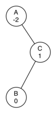
Below shows us that after the left rotation we are now out of balance the other way. If we do a right rotation to correct the situation we are right back where we started!

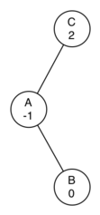
To correct this problem we must use the following set of rules:

1. If a subtree needs a left rotation to bring it into balance, first check the balance factor of the right child. If the right child is left-heavy, then do a right rotation on right child followed by the original left rotation.

2. If a subtree needs a right rotation to bring it into balance, first check the balance factor of the left child. If the left child is right-heavy, then do a left rotation on the left child followed by the original right rotation.

Figure below shows how these rules solve the dilemma we encountered. Starting with a right rotation around node C puts the tree in a position where the left rotation around A brings the entire subtree back into balance.

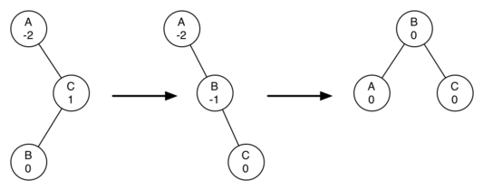
The code that implements these rules can be found in our rebalance method:

def rebalance(self, node):
    if node.balance_factor < 0:
        if node.right_child.balance_factor > 0:
            self.rotate_right(node.right_child)
            self.rotate_left(node)
        else:
            self.rotate_left(node)
    elif node.balance_factor > 0:
        if node.left_child.balance_factor < 0:
            self.rotate_left(node.left_child)
            self.rotate_right(node)
        else:
            self.rotate_right(node)

By keeping the tree in balance at all times, we can ensure that the get method will run in order $O(log_2(n))$ time. But the question is at what cost to our put method? Let us break this down into the operations performed by put().

Since a new node is inserted as a leaf, updating the balance factors of all the parents will require a maximum of $log_2(n)$ operations, one for each level of the tree. If a subtree is found to be out of balance, a maximum of two rotations are required to bring the tree back into balance. But each of the rotations works in $O(1)$ time, so even our put operation remains $O(log_2(n))$.

At this point we have implemented a functional AVL tree, unless you need the ability to delete a node. We leave the deletion of the node and subsequent updating and rebalancing as an exercise for you.

display_quiz(path+"avl.json", max_width=800)

from pythonds3.trees import AVLTree
#Create a new AVL Tree
avl_tree = AVLTree()

# Insert elements into the AVL Tree
avl_tree.put(1, 'one')
avl_tree.put(2, 'two')
avl_tree.put(3, 'three')
avl_tree.put(4, 'four')
avl_tree.put(5, 'five')

# Output the root of the tree
print(f"Root of the AVL Tree: {avl_tree._root.key}, Value: {avl_tree._root.value}")

# Check the balance factor of the root
print(f"Balance Factor of the root: {avl_tree._root.balance_factor}")

# Perform a left rotation (manually for demonstration purposes)
avl_tree.rotate_left(avl_tree._root)

# Re-check the root after rotation
print(f"New root after left rotation: {avl_tree._root.key}, Value: {avl_tree._root.value}")
print(f"Balance Factor of the root: {avl_tree._root.balance_factor}")

Root of the AVL Tree: 2, Value: two
Balance Factor of the root: -1
New root after left rotation: 4, Value: four
Balance Factor of the root: 1

6.19. Summary of Map ADT Implementations

Over the past two chapters we have looked at several data structures that can be used to implement the map abstract data type: a binary search on a list, a hash table, a binary search tree, and a balanced binary search tree. To conclude this section, let’s summarize the performance of each data structure for the key operations defined by the map ADT:

operation	Sorted List	Hash Table	Binary Search Tree	AVL Tree
put()	$O(n)$	$O(1)$	$O(n)$	$O(\log_2{n})$
get()	$O(\log_2{n})$	$O(1)$	$O(n)$	$O(\log_2{n})$
in()	$O(\log_2{n})$	$O(1)$	$O(n)$	$O(\log_2{n})$
del()	$O(1)$	$O(1)$	$O(n)$	$O(\log_2{n})$

from jupytercards import display_flashcards
fpath= "https://raw.githubusercontent.com/phonchi/nsysu-math208/refs/heads/main/extra/flashcards/"
#fpath= "flashcards/"
display_flashcards(fpath + 'ch9.json')

References

1. Textbook CH6

Key terms

1. Trees: A hierarchical data structure consisting of nodes, where each node contains data and references to child nodes, facilitating efficient data organization and retrieval.

2. Node: A fundamental part of a tree that stores data and contains references to other nodes (children). Each node in a tree can represent a data point or a position in the structure.

3. Edge: The connection between two nodes in a tree, representing the relationship or link from a parent node to a child node.

4. Root: The topmost node in a tree, from which all other nodes descend. It does not have a parent node.

5. Path: A sequence of nodes and edges connecting a node with a descendant, showing the route from one node to another within the tree.

6. Children: Nodes that are directly connected and descend from another node (the parent) within a tree.

7. Parent: The converse of a child in a hierarchical tree, this node has one or more nodes (children) directly under it.

8. Sibling: Nodes that share the same parent in a tree, thus residing at the same level and having the same parent.

9. Subtree: A portion of a tree structure consisting of a node and all its descendants, forming a tree itself within the larger tree.

10. Leaf node: A node with no children, representing an endpoint or "leaf" of a tree.

11. Level: The layer or depth of a node within a tree, starting at zero for the root node, with each step down increasing the level by one.

12. Height: The total number of levels in a tree, or the length of the longest path from the root to a leaf node.

13. Binary Tree: A type of tree where each node has at most two children, typically referred to as the left and right children.

14. List of Lists: A method for implementing a tree using a nested list structure, where each list can represent a node and its children.

15. Nodes and References: A common method for implementing trees in which each node contains its data and references (links) to its children.

16. Parse Tree: A tree that represents the syntactic structure of a string according to some formal grammar, used in compilers and parsers for understanding programming languages or data.

17. Expression Tree: A binary tree specifically used to represent and evaluate expressions, where each internal node denotes an operator and each leaf node denotes an operand.

18. Preorder: A way to traverse a tree where each node is processed before its child nodes (root, left, right).

19. Postorder: A tree traversal method where each node is processed after its child nodes (left, right, root).

20. Inorder: A traversal technique used primarily in binary trees where nodes are processed in the order left-child, root, right-child.

21. Priority Queue: An abstract data type in which each element is associated with a priority, and elements are served according to their priority.

22. Binary Heap: A binary tree-based data structure that satisfies the heap property, where each node is either greater than or equal to or less than or equal to each of its children, according to a comparator.

23. Complete Binary Tree: A binary tree in which every level, except possibly the last, is completely filled, and all nodes are as far left as possible.

24. Heap Structure Property: A property of a heap that mandates the tree be a complete binary tree, ensuring optimal balance for quick insertions and deletions.

25. Heap Order Property: The key property of a heap that maintains a specific order between a node and its children, typically a max-heap or min-heap order.

26. Max-Heap: A max-heap is a specialized tree-based data structure in which the value of each node is greater than or equal to the values of its children. This ensures that the highest value is always at the root, making max-heaps ideal for applications where quick access to the largest element is necessary, such as priority queues.

27. Min-Heap: A min-heap is the opposite of a max-heap. In a min-heap, each node's value is less than or equal to the values of its children. This arrangement ensures that the smallest value is always at the root, which is beneficial for applications needing quick access to the smallest element, such as implementing efficient priority queues and Dijkstra's shortest path algorithm.

28. Binary Search Tree (BST): A binary tree in which each node has a key greater than all the keys in its left subtree and less than those in its right subtree.

29. BST Property: The defining characteristic of a binary search tree, where for every node, all elements in the left subtree are less than the node and all in the right are greater.

30. Successor: The node that comes immediately after a given node in the order of an inorder traversal of a binary search tree.

31. Generator Function: A type of function that returns an iterator. It allows the function to yield values one at a time, pausing and resuming its execution.

32. Balanced Binary Search Tree: A type of binary search tree that maintains a low height by automatically adjusting the tree during insertions and deletions to ensure minimal path length.

33. Balance Factor: In AVL trees, this is the difference in the heights of the left and right subtrees for any node, used to maintain tree balance.

34. AVL Tree: A self-balancing binary search tree where the height of the left and right subtrees can only differ by at most one for all nodes, ensuring $O(\log n)$ time complexity for search, insert, and delete operations.