Graphs and Graph Algorithms

|

|
The Graph Abstract Data Type
Breadth-First Search
Depth-First Search
Shortest Path Problems
Minimum Spanning Tree
Introduction
Graphs can be used to represent many interesting things about our world, including systems of roads, airline flights, how the internet is connected, or even the sequence of classes you must take.
We will see in this chapter that once we have a good representation for a problem, we can use some standard graph algorithms to solve what otherwise might seem to be a very difficult problem!
A graph is just like a road map. If you have ever used one of the internet map sites, you know that a computer can find the shortest, quickest, or easiest path from one place to another.
9.2. Vocabulary and Definitions
- Vertex: A vertex (also called a node) is a fundamental part of a graph. It can have a name, which we will call the key. A vertex may also have additional information. We will call this additional information the value or the payload.
- Edge: An edge (also called an arc) is another fundamental part of a graph. An edge connects two vertices to show that there is a relationship between them. Edges may be one-way or two-way. If the edges in a graph are all one-way, we say that the graph is a directed graph, or a digraph.
- Weight: Edges may be weighted to show that there is a cost to go from one vertex to another, which we call edge cost. For example, in a graph of roads that connect one city to another, the weight on the edge might represent the distance between the two cities.
A graph can be represented by $G =(V,E)$. For the graph $G$, $V$ is a set of vertices and $E$ is a set of edges. Each edge is a pair $(v,w)$ where $v, w \in V$. A weighted edge adds a third component, the weight. A subgraph $s$ is a set of edges $e$ and vertices $v$ such that $e \subset E$ and $v \subset V$.
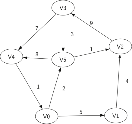
The above is a simple weighted digraph. Formally we can represent this graph as the set of six vertices:
$$V = \left\{ v_0, v_1, v_2, v_3, v_4, v_5 \right\}$$
and the set of nine edges:
$$\begin{split}E = \left\{ \begin{array}{l}(v_0, v_1, 5), (v_1, v_2, 4), (v_2, v_3, 9), \\ (v_3, v_4, 7), (v_4, v_0, 1), (v_0, v_5, 2), \\ (v_5, v_4, 8), (v_3, v_5, 3), (v_5, v_2, 1) \end{array} \right\}\end{split}$$
The example graph helps illustrate two other key graph terms:
- Path: A path in a graph is a sequence of distinct vertices $w_1, w_2, \ldots, w_n$ such that $(w_i, w_{i+1}) \in E$ for all $1 \le i \le n-1$. The unweighted path length is the number of edges, $n-1$; the weighted path length is the sum of the weights of all edges in the path. For example, the path from $v_3$ to $v_1$ is $(v_3, v_4, v_0, v_1)$. (A more general sequence that allows repeated vertices is called a walk.)
- Cycle: A cycle is a closed sequence $(w_1, w_2, \ldots, w_n, w_1)$ where $w_1, \ldots, w_n$ are distinct vertices and consecutive vertices are connected by an edge. For example, $(v_5, v_2, v_3, v_5)$ is a cycle. A graph with no cycles is called an acyclic graph, and a directed graph with no cycles is called a directed acyclic graph (DAG). We will see that many important problems can be solved efficiently if they can be modeled as a DAG!
A tree is a connected, acyclic, undirected graph. In other words, there is a path between every pair of vertices, and the graph contains no cycles. We will explore different types of trees in detail in the next chapter!
9.3. The Graph Abstract Data Type
Note that vertices may be either connected to each other or isolated. Edges join two vertices and may be weighted.
Graph(): creates an empty graph.setVertex(key): inserts a missing vertex. If the key already exists, it is a no-op, so existing edges and traversal state are preserved.
addEdge(fromKey, toKey): adds a directed, zero-weight edge and creates missing endpoint vertices.addEdge(fromKey, toKey, weight): adds or updates a weighted directed edge.
vertices.find(key)orvertices.count(key): tests whether a key exists.A range-based loop over
verticesvisits all key/Vertexpairs.
The compact course header intentionally exposes the ordered vertices map (map<string, Vertex>), so membership tests and iteration use the standard map operations above.
Now that we have looked at the definition for the graph ADT, there are several ways we can implement it. There are two well-known implementations of a graph, the adjacency matrix and the adjacency list.
9.4. An Adjacency Matrix
One of the easiest ways to implement a graph is to use a two-dimensional matrix. Each of the rows and columns represents a vertex in the graph. The value that is stored in the cell at the intersection of row $v$ and column $w$ indicates if there is an edge.
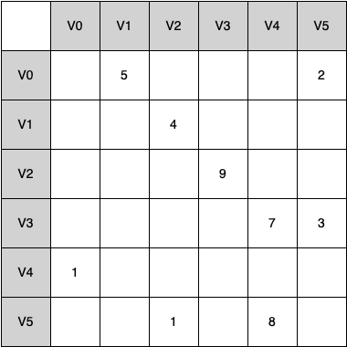
When two vertices are connected by an edge, we say that they are adjacent and the value in each cell represents the weight. The advantage of the adjacency matrix is that it is simple, and for small graphs it is easy to see which nodes are connected to other nodes. However, we can say that this matrix is sparse. A matrix is not a very efficient way to store sparse data.
The adjacency matrix is thus a good implementation for a graph when the number of edges is large. Since there is one row and one column for every vertex in the graph, the number of edges required to fill the matrix is $|V|^2$.
However, there are few real problems that approach this sort of connectivity. The problems we will look at in this chapter all involve graphs that are sparsely connected!
9.5. An Adjacency List
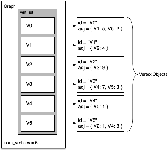
A sparse graph is stored as an adjacency structure. In our C++ implementation, Graph::vertices is a map<string, Vertex>, and each Vertex::neighbors is a map<string, int> from neighbor key to edge weight.
In the C++ implementation, each Vertex stores map<string, int> neighbors: keys identify adjacent vertices and values store edge weights.
An adjacency structure uses $O(|V|+|E|)$ storage and lists the neighbors of $v$ in $O(\deg(v))$ time. Our ordered-map implementation additionally makes vertex and edge-key lookup $O(\log |V|)$ and $O(\log \deg(v))$, respectively; those logarithmic factors come from std::map, not from the graph ADT itself.
display_quiz(quiz_path+"graph.json", max_width=800)
9.6. Implementation
class Vertex {
    public:
        string key;
        map<string, int> neighbors;   // neighbor key -> edge weight
        string color = "white";       // traversal state used by BFS/DFS
        int distance = INT_MAX;
        string previous = "";

        Vertex() {}
        Vertex(string k) {
            key = k;
        }

        int getNeighbor(string other) {
            if (neighbors.count(other)) {
                return neighbors[other];
            }
            return -1;   // no such edge
        }
        void setNeighbor(string other, int weight = 0) {
            neighbors[other] = weight;
        }
};
Each Vertex uses map<string, int> neighbors to associate a neighbor key with an edge weight. setNeighbor(other, weight) inserts or updates that mapping, and getNeighbor(other) retrieves the weight when the edge exists. The header graph.hpp used by the examples has the same members but leaves out these two convenience methods; its code reads and writes neighbors directly.
class Graph {
    public:
        map<string, Vertex> vertices;

        void setVertex(string key) {
            if (vertices.count(key) == 0) vertices.emplace(key, Vertex(key));
        }
        void addEdge(string fromVert, string toVert, int weight = 0) {
            if (vertices.count(fromVert) == 0) setVertex(fromVert);
            if (vertices.count(toVert) == 0) setVertex(toVert);
            vertices[fromVert].neighbors[toVert] = weight;
        }
        bool contains(string key) {
            return vertices.count(key) > 0;
        }
};
The Graph class also uses map<string, Vertex> vertices to map vertex keys to objects. C++ range-based loops iterate over its key/value pairs; vertices.count(key) tests membership; graph.hpp has no contains() and calls vertices.count(key) directly.
Now let us define the graph seen earlier. We create six vertices numbered 0 through 5, then inspect the vertices map. Each key names one Vertex object.
#include <iostream>
#include "pythonds3/cppds/graph.hpp"   // Vertex + Graph (md listing above)
using namespace std;

int main() {
    Graph g;
    for (int i = 0; i < 6; i++) {
        g.setVertex(to_string(i));
    }
    for (auto& p : g.vertices) {
        cout << "Vertex(" << p.first << ") ";
    }
    cout << endl;
    return 0;
}
Vertex(0) Vertex(1) Vertex(2) Vertex(3) Vertex(4) Vertex(5)
Next, we add the edges that connect the vertices together. Finally, a nested loop verifies that each edge in the graph is properly stored:
#include <iostream>
#include "pythonds3/cppds/graph.hpp"
using namespace std;

int main() {
    Graph g;
    g.addEdge("0","1",5); g.addEdge("0","5",2); g.addEdge("1","2",4);
    g.addEdge("2","3",9); g.addEdge("3","4",7); g.addEdge("3","5",3);
    g.addEdge("4","0",1); g.addEdge("5","4",8); g.addEdge("5","2",1);

    for (auto& p : g.vertices)
        for (auto& n : p.second.neighbors)
            cout << "(" << p.first << "," << n.first << "," << n.second << ") ";
    cout << endl;
    return 0;
}
(0,1,5) (0,5,2) (1,2,4) (2,3,9) (3,4,7) (3,5,3) (4,0,1) (5,2,1) (5,4,8)
9.7. The Word Ladder Problem
To begin our study of graph algorithms let's consider the following puzzle called a word ladder: transform the word FOOL into the word SAGE. In a word ladder puzzle you must make the change occur gradually by changing one letter at a time.
At each step you must transform one word into another word; you are not allowed to transform a word into a non-word. The following sequence of words shows one possible solution to the problem posed above:
FOOL
POOL
POLL
POLE
PALE
SALE
SAGE
There are many variations of the word ladder puzzle. For example you might be given a particular number of steps in which to accomplish the transformation, or you might need to use a particular word. In this section, we are interested in figuring out the smallest number of transformations needed to turn the starting word into the ending word.
Here is an outline of where we are going:
- Represent the relationships between the words as a graph.
- Use the graph algorithm known as breadth-first search to find an efficient path from the starting word to the ending word.
9.8. Building the Word Ladder Graph
Our first problem is to figure out how to turn a large collection of words into a graph. What we would like is to have an edge from one word to another if the two words are only different by a single letter.
If we can create such a graph, then any path from one word to another is a solution to the word ladder puzzle!
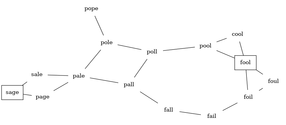
Let's start with the assumption that we have a list of words that are all the same length. As a starting point, we can create a vertex in the graph for every word in the list.
To figure out how to connect the words, we could compare each word in the list with every other. When we compare we are looking to see how many letters are different. If the two words in question are different by only one letter, we can create an edge between them in the graph.
For a small set of words that approach would work fine. However, let's suppose we have a list of 5,110 words. Roughly speaking, comparing one word to every other word on the list is an $O(n^2)$ algorithm. For 5,110 words, is more than 26 million comparisons!
We can do much better by assuming that we have a number of buckets, each labeled with a four-letter word, except that one of the letters on the label has been replaced by an underscore. As we process a list of words, we compare each word with each bucket using the underscore (_) as a wildcard.
Every time we find a matching bucket we put the word in that bucket, so that both POPE and POPS would both go into the POP_ bucket. Once we have all the words in the appropriate buckets, we know that all the words in each bucket must be connected!
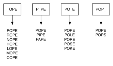
The reusable implementation used by the executable examples is split between pythonds3/cppds/graph.hpp (data structure) and pythonds3/cppds/graph_algos.hpp (algorithms). The longer graphs/adjacency_graph.cpp file is retained as a standalone reference listing.
Graph buildGraph(vector<string> words) {
    map<string, set<string>> buckets;
    Graph theGraph;

    // create buckets of words that differ by one letter
    for (string word : words) {
        for (unsigned i = 0; i < word.length(); i++) {
            string bucket = word.substr(0, i) + "_" + word.substr(i + 1);
            buckets[bucket].insert(word);
        }
    }

    // add edges between different words in the same bucket
    for (auto& pair : buckets) {
        for (const string& word1 : pair.second) {
            for (const string& word2 : pair.second) {
                if (word1 != word2) {
                    theGraph.addEdge(word1, word2);
                }
            }
        }
    }
    return theGraph;
}
The bucket scheme uses map<string, set<string>>: each wildcard label is a map key and its set contains the words sharing that pattern.
The 5,110-word adjacency matrix would contain $5{,}110^2=26{,}112{,}100$ cells. buildGraph() stores 53,286 directed adjacency entries (26,643 undirected word pairs), only about 0.20% of those cells, so the graph is very sparse.
9.9. Implementing Breadth First Search
With the graph constructed we can now turn our attention to the algorithm we will use to find the shortest solution to the word ladder problem. The graph algorithm we are going to use is called the breadth-first search (BFS), and it is one of the easiest algorithms for searching a graph!
Given a starting vertex $s$ of a graph, a breadth first search proceeds by exploring edges in the graph to find all the vertices in $G$ for which there is a path from $s$.
The remarkable thing about a breadth-first search is that it finds all the vertices that are a distance $k$ from $s$ before it finds any vertices that are a distance $k+1$.
To keep track of its progress, BFS colors each of the vertices white, gray, or black. All the vertices are initialized to white when they are constructed. A white vertex is an undiscovered vertex. When a vertex is initially discovered it is colored gray, and when BFS has completely explored a vertex it is colored black.
This means that once a vertex is colored black, it has no white vertices adjacent to it. A gray node, on the other hand, may have some white vertices adjacent to it, indicating that there are still additional vertices to explore.
The bfs() shown below uses the adjacency list graph representation we developed earlier. In addition it uses a Queue, a crucial point as we will see, to decide which vertex to explore next.
void bfs(Graph& g, string startKey) {
    for (auto& p : g.vertices) {   // reset every vertex
        p.second.color = "white"; p.second.distance = INT_MAX; p.second.previous = "";
    }
    g.vertices[startKey].distance = 0;
    g.vertices[startKey].color = "gray";
    queue<string> vertQueue;
    vertQueue.push(startKey);
    while (!vertQueue.empty()) {
        string currentKey = vertQueue.front();
        vertQueue.pop();
        Vertex& current = g.vertices[currentKey];
        for (auto& n : current.neighbors) {
            Vertex& neighbor = g.vertices[n.first];
            if (neighbor.color == "white") {
                neighbor.color = "gray";
                neighbor.distance = current.distance + 1;
                neighbor.previous = currentKey;
                vertQueue.push(n.first);
            }
        }
        current.color = "black";
    }
}
The BFS algorithm uses three extra data members of the Vertex class: distance, previous, and color. They are public members, so the algorithm reads and updates them directly.
Before each BFS run, every vertex is reset to white, unreachable distance (INT_MAX), and no predecessor (empty string). BFS then sets start.distance = 0, paints start gray before enqueueing it, and explores vertices from the front of a FIFO queue.
As each node on the adjacency list is examined, its color is checked. If it is white four things happen:
The new unexplored vertex
neighboris colored gray.The predecessor of
neighboris set to the current nodecurrent.
The distance to
neighboris set tocurrent.distance + 1.neighboris added to the end of the queue. This schedules it after every vertex already waiting at the same or an earlier layer.
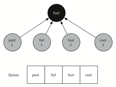
Starting from FOOL we take all nodes that are adjacent to FOOL and add them to the queue. The adjacent nodes include POOL, FOIL, FOUL, and COOL. Each of these nodes are new nodes to expand.
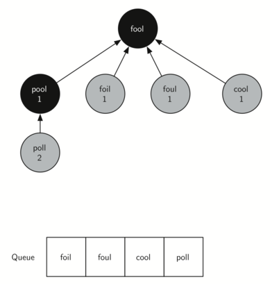
In the next step bfs removes the next node (POOL) from the front of the queue and repeats the process for all of its adjacent nodes.
However, when bfs examines the node COOL, it finds that the color of COOL has already been changed to gray. This indicates that there is a shorter path to COOL and that COOLis already on the queue for further expansion. The only new node added to the queue while examining POOL is POLL.
The next vertex on the queue is FOIL. The only new node that FOIL can add to the tree is FAIL. As bfs continues to process the queue, neither of the next two nodes adds anything new to the queue or the tree. Below shows the tree and the queue after expanding all the vertices on the second level of the tree:
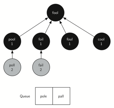
You should continue to work through the algorithm on your own so that you are comfortable with how it works. Figure below shows the final breadth-first search tree after all the vertices.
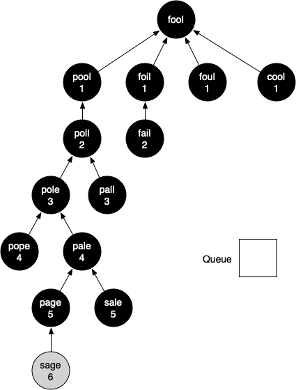
The amazing thing about the breadth-first search solution is that we have not only solved the FOOL–SAGE problem we started out with, but we have solved many other problems along the way.
We can start at any vertex in the breadth-first search tree and follow the predecessor arrows back to the root to find the shortest word ladder from any word back to FOOL.
void traverse(Graph& g, string startingKey) {
    string current = startingKey;
    while (current != "") {
        cout << current;
        if (g.vertices[current].previous != "") {
            cout << "->";
        }
        current = g.vertices[current].previous;
    }
    cout << endl;
}
#include <iostream>
#include "pythonds3/cppds/graph_algos.hpp"   // buildGraph + bfs + traverse
using namespace std;

int main() {
    Graph g = buildGraph({"fool", "cool", "pool", "poll", "pole",
                         "pall", "fall", "fail", "foil", "foul",
                         "pope", "pale", "sale", "sage", "page"});
    bfs(g, "fool");
    traverse(g, "sage");
    return 0;
}
sage->page->pale->pall->poll->pool->fool
#include <iostream>
#include "pythonds3/cppds/graph_algos.hpp"
using namespace std;

int main() {
    Graph g = buildGraph({"fool", "cool", "pool", "poll", "pole",
                         "pall", "fall", "fail", "foil", "foul",
                         "pope", "pale", "sale", "sage", "page"});
    bfs(g, "fool");
    for (auto& p : g.vertices)   // word(distance from fool)
        cout << p.first << "(" << p.second.distance << ") ";
    cout << endl;
    return 0;
}
cool(1) fail(2) fall(3) foil(1) fool(0) foul(1) page(5) pale(4) pall(3) pole(3) poll(2) pool(1) pope(4) sage(6) sale(5)
9.10. Breadth First Search Analysis
Let's analyze the run time performance of the breadth-first search algorithm. The first thing to observe is that the while loop is executed, at most, one time for each vertex in the graph (up to $|V|$ iterations). You can see that this is true because a vertex must be white before it can be examined and added to the queue.
This gives us $O(|V|)$ for the while loop. The for loop, which is nested inside the while, is executed at most once for each edge in the graph (up to $|E|$ iterations). The reason is that every vertex is dequeued at most once and we examine an edge from node $u$ to node $v$ only when node $u$ is dequeued.
This gives us $O(|E|)$ for the for loop. Combining the two loops gives us $O(|V| + |E|)$.
Of course doing the breadth-first search is only part of the task. Following the links from the starting node to the goal node is the other part of the task.
The worst case for this would be if the graph was a single long chain. In this case traversing through all of the vertices would be $O(|V|)$. The normal case is going to be some fraction of $|V|$.
Finally, at least for this problem, there is the time required to build the initial graph.
9.11. The Knight's Tour Problem
Another classic problem that we can use to illustrate a second common graph algorithm is called the knight's tour. The knight's tour puzzle is played on a chess board with a single chess piece, the knight.
The object of the puzzle is to find a sequence of moves that allow the knight to visit every square on the board exactly once. One such sequence is called a tour.
The upper bound on the number of possible legal tours for an $8 \times 8$ chessboard is known to be $10^{35}$; however, there are even more possible dead ends.
Although researchers have studied many different algorithms to solve the knight's tour problem, a graph search is one of the easiest to understand and program. Once again we will solve the problem using two main steps:
- Represent the legal moves of a knight on a chessboard as a graph.
- Use a graph algorithm to find a path of length $rows \times columns - 1$ where every vertex on the graph is visited exactly once!
9.12. Building the Knight's Tour Graph
To represent the knight's tour problem as a graph we will use the following two ideas: each square on the chessboard can be represented as a node in the graph and each legal move by the knight can be represented as an edge in the graph.
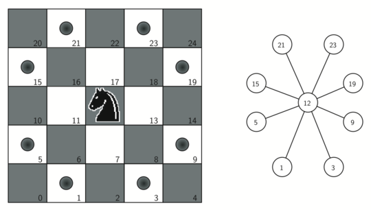
Graph knightGraph(int boardSize) {
    Graph ktGraph;
    for (int row = 0; row < boardSize; row++) {
        for (int col = 0; col < boardSize; col++) {
            int nodeId = row * boardSize + col;
            for (auto& move : genLegalMoves(row, col, boardSize)) {
                int otherNodeId = move.first * boardSize + move.second;
                ktGraph.addEdge(to_string(nodeId), to_string(otherNodeId));
            }
        }
    }
    return ktGraph;
}
The knightGraph() function makes one pass over the board. At each square it calls genLegalMoves() to produce the legal destination coordinates, then stores one directed adjacency entry for each legal move.
All legal moves are then converted into edges in the graph. Each location on the board is converted into a linear vertex number.
The genLegalMoves() takes the position of the knight on the board and generates each of the eight possible moves, making sure those moves are still within the board:
vector<pair<int, int>> genLegalMoves(int row, int col, int boardSize) {
    vector<pair<int, int>> newMoves;
    vector<pair<int, int>> moveOffsets = {
        {-1, -2}, {-1, 2}, {-2, -1}, {-2, 1},
        {1, -2},  {1, 2},  {2, -1},  {2, 1}};
    for (auto& off : moveOffsets) {
        int newRow = row + off.first;
        int newCol = col + off.second;
        if (0 <= newRow && newRow < boardSize && 0 <= newCol && newCol < boardSize) {
            newMoves.push_back({newRow, newCol});
        }
    }
    return newMoves;
}
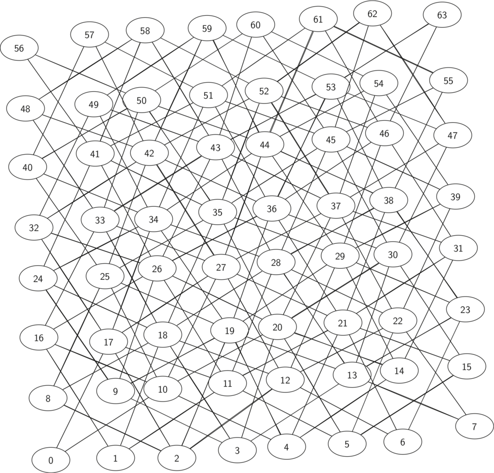
The figure shows the complete graph of possible moves on an $8 \times 8$ board. There are exactly 336 edges in the graph. Notice that the vertices corresponding to the edges of the board have fewer connections (legal moves) than the vertices in the middle of the board.
The $8\times8$ adjacency matrix has 4,096 cells. The representation stores 336 directed adjacency arcs (each legal undirected move appears in both directions), equivalent to 168 undirected edges, so only 8.2% of the matrix cells would be occupied.
9.13. Implementing Knight's Tour
The search algorithm we will use to solve the knight's tour problem is called depth-first search (DFS). Whereas the breadth-first search algorithm builds a search tree one level at a time, a depth-first search creates a search tree by exploring one branch of the tree as deeply as possible.
We will look at two algorithms that implement DFS. The first algorithm we will look at specifically solves the knight's tour problem by explicitly forbidding a node to be visited more than once.
The second implementation is more general, but allows nodes to be visited more than once as the tree is constructed. The second version is used in subsequent sections to develop additional graph algorithms.
The depth-first exploration of the graph is exactly what we need in order to find a path through 64 vertices (one for each square on the chessboard) and 63 edges.
We will see that when the depth-first search algorithm finds a dead end (a place in the graph where there are no more moves possible) it backs up the tree to the next deepest vertex that allows it to make a legal move.
The knightTour() function takes four main arguments: n, the current depth; path, a vector<string> of visited vertex keys; uKey, the vertex being explored; and limit, the final path depth.
bool knightTour(int n, vector<string>& path, string uKey, int limit, Graph& g) {
    g.vertices[uKey].color = "gray";
    path.push_back(uKey);
    if (n < limit) {
        bool done = false;
        for (auto& nb : g.vertices[uKey].neighbors) {
            if (done) break;
            if (g.vertices[nb.first].color == "white") {
                done = knightTour(n + 1, path, nb.first, limit, g);
            }
        }
        if (!done) {   // prepare to backtrack
            path.pop_back();
            g.vertices[uKey].color = "white";
        }
        return done;
    }
    return true;
}
The function is recursive. If the path has reached the required depth, it returns true. Otherwise it examines an unvisited neighbor, recurses one level deeper, and returns whether that choice eventually completes the tour.
DFS also uses colors to keep track of which vertices in the graph have been visited. Unvisited vertices are colored white, and visited vertices are colored gray. If all neighbors of a particular vertex have been explored and we have not yet reached our goal length of 64 vertices, we have reached a dead end and must backtrack.
Backtracking happens when a recursive call returns false: the last key is removed from path and that vertex is painted white again. The recursive call stack records the choices that remain to be reconsidered.
When a recursive call returns false, the loop proceeds to the next white neighbor. If none completes the tour, the current call removes its vertex from path, resets it to white, and returns false.
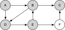
For a small trace, assume iteration over the neighbors map follows key order. We call knightTour(1, path, "A", 6, g) and watch the recursive choices and backtracking.
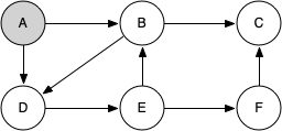
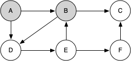
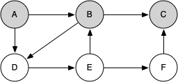
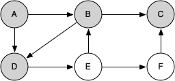
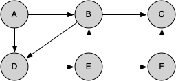
knightTour() starts at A. Its adjacent vertices are B and D, so ordered map iteration tries B first. From B it tries C before D and reaches a dead end.
Node C is a dead end with no white neighbor, so its call returns false, resets C to white, and backtracks to B. The search can then try D, the next neighbor.
Later the search reaches C only after every required vertex is already in the path. The base-case test succeeds and returns true, which propagates through the recursive calls.
When the search succeeds, the vector<string> path contains [A, B, D, E, F, C], the order that visits each vertex exactly once.
#include <iostream>
#include "pythonds3/cppds/graph_algos.hpp"   // genLegalMoves + knightGraph + knightTour
using namespace std;

int main() {
    // brute force: 5x5 board - 8x8 without the heuristic takes far too long!
    int boardSize = 5;
    Graph ktGraph = knightGraph(boardSize);
    vector<string> path;
    bool finished = knightTour(1, path, "0", boardSize * boardSize, ktGraph);
    if (finished) printBoard(path, boardSize);   // squares show the move number
    else cout << "No path found." << endl;
    return 0;
}
0 5 14 11 20
15 10 19 6 13
4 1 12 21 18
9 16 23 2 7
24 3 8 17 22
Instead of a matplotlib figure, we print the board as a grid where each square shows the move number on which the knight visits it — 0 is the start and 24 (or 63) the final move.
For an 8×8 board this plain depth-first search is hopeless — the next section explains why, and the Warnsdorff heuristic below fixes it.
Each vertex of the knight graph also carries the usual BFS/DFS bookkeeping state (color, previous), which the tour uses to avoid revisiting squares.
9.14. Knight's Tour Analysis
knightTour() is very sensitive to the method you use to select the next vertex to visit. For example, on a $5 \times 5$ board you can produce a path in about 1.5 seconds on a reasonably fast computer. But what happens if you try an $8 \times 8$ board? In this case, depending on the speed of your computer, you may have to wait up to several minutes to get the results!
The reason for this is that the knight's tour problem as we have implemented it so far is an exponential algorithm of size $O(k^N)$, where $N$ is the number of squares on the chess board, and $k$ is a small constant.
We can use a tree to help us undertand this point. The root of the tree represents the starting point of the search. From there the algorithm generates and checks each of the possible moves the knight can make.
As we have noted before, the number of moves possible depends on the position of the knight on the board. In the corners there are only two legal moves, on the squares adjacent to the corners there are three, and in the middle of the board there are eight.
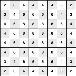
At the next level of the tree there are once again between two and eight possible next moves from the position we are currently exploring. The number of possible positions to examine corresponds to the number of nodes in the search tree.
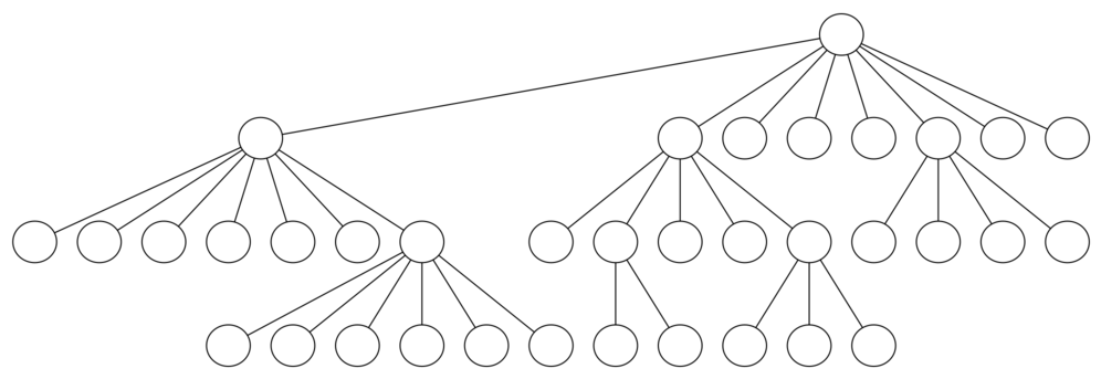
For a tree with nodes that may have up to eight children, the number of nodes is large. Because the branching factor of each node is variable, we could estimate the number of nodes using an average branching factor. The important thing to note is that this algorithm is exponential: $\frac{k^{N+1}-1}{k-1}$, where $k$ is the average branching factor for the board.
Let's look at how rapidly this grows! For a board that is $5 \times 5$ the tree will be 25 levels deep. The average branching factor is $k=3.8$ so the number of nodes in the search tree is on the order of $k^N$: $3.8^{25} \approx 3.1 \times 10^{14}$.
For a $6 \times 6$ board, $k = 4.4$, there are on the order of $4.4^{36} \approx 1.5 \times 10^{23}$ nodes, and for a regular $8 \times 8$ chess board, $k = 5.25$, on the order of $5.25^{64} \approx 1.2 \times 10^{46}$!
Of course, since there are multiple solutions to the problem we won't have to explore every single node, but the fractional part of the nodes we do have to explore is just a constant multiplier which does not change the exponential nature of the problem.
orderByAvail() orders candidate neighbor keys by their number of remaining white neighbors. Trying the least constrained count first is Warnsdorff's rule and makes the $8\times8$ case practical, without changing the exponential worst-case guarantee.
vector<string> orderByAvail(Graph& g, string uKey) {
    vector<pair<int, string>> resList;
    for (auto& nb : g.vertices[uKey].neighbors) {
        if (g.vertices[nb.first].color == "white") {
            int c = 0;
            for (auto& w : g.vertices[nb.first].neighbors) {
                if (g.vertices[w.first].color == "white") {
                    c++;
                }
            }
            resList.push_back({c, nb.first});
        }
    }
    sort(resList.begin(), resList.end());   // fewest onward moves first
    vector<string> result;
    for (auto& p : resList) {
        result.push_back(p.second);
    }
    return result;
}
You might think this is really counterproductive; why not select the node that has the most available moves?
You can try that approach easily by running the program yourself and inserting the line reverse(resList.begin(), resList.end()); right after the sort.
The problem with using the vertex with the most available moves as your next vertex on the path is that it tends to have the knight visit the middle squares early on in the tour!
When this happens it is easy for the knight to get stranded on one side of the board where it cannot reach unvisited squares on the other side of the board. On the other hand, visiting the squares with the fewest available moves first pushes the knight to visit the squares around the edges of the board first.
This ensures that the knight will visit the hard-to-reach corners early and can use the middle squares to hop across the board only when necessary. Utilizing this kind of knowledge to speed up an algorithm is called a heuristic. This particular heuristic is called Warnsdorff's algorithm.
bool knightTourWarnsdorff(int n, vector<string>& path, string uKey, int limit, Graph& g) {
    g.vertices[uKey].color = "gray";
    path.push_back(uKey);
    if (n < limit) {
        bool done = false;
        for (string nbKey : orderByAvail(g, uKey)) {   // Warnsdorff order
            if (done) break;
            if (g.vertices[nbKey].color == "white") {
                done = knightTourWarnsdorff(n + 1, path, nbKey, limit, g);
            }
        }
        if (!done) {
            path.pop_back();
            g.vertices[uKey].color = "white";
        }
        return done;
    }
    return true;
}
#include <iostream>
#include "pythonds3/cppds/graph_algos.hpp"   // orderByAvail + knightTourWarnsdorff
using namespace std;

int main() {
    int boardSize = 8;   // with the heuristic, 8x8 finishes instantly
    Graph ktGraph = knightGraph(boardSize);
    vector<string> path;
    bool finished = knightTourWarnsdorff(1, path, "0", boardSize * boardSize, ktGraph);
    if (finished) printBoard(path, boardSize);
    else cout << "No path found." << endl;
    return 0;
}
0 3 40 19 38 5 42 21
33 18 1 4 41 20 37 6
2 51 34 39 36 55 22 43
17 32 49 62 53 44 7 56
50 13 52 35 48 57 54 23
31 16 61 58 63 26 45 8
12 59 14 29 10 47 24 27
15 30 11 60 25 28 9 46
With Warnsdorff's heuristic the 8×8 tour completes in milliseconds — a dramatic contrast with the exponential brute-force search.
9.15. General Depth First Search
The knight's tour uses depth-first backtracking to search for one simple path that visits every square. General DFS has a different goal: it explores every reachable vertex and records a depth-first tree; running it from each remaining white vertex produces a depth-first forest, whose trees may have many branches.
The more general depth-first search is actually easier. Its goal is to search as deeply as possible, connecting as many nodes in the graph as possible and branching where necessary.
It is even possible that a depth-first search will create more than one tree. When the depth-first search algorithm creates a group of trees we call this a depth-first forest.
As with the breadth-first search, our depth-first search makes use of predecessor links to construct the tree. In addition, the depth-first search records two timestamps for every vertex: its discovery and closing times, stored in the DFSGraph members discovery and closing.
- The discovery time tracks the number of steps in the algorithm before a vertex is first encountered.
- The closing time is the number of steps in the algorithm before a vertex is colored black.
As we will see after looking at the algorithm, the discovery and closing times of the nodes provide some interesting properties we can use in later algorithms.
class DFSGraph : public Graph {
    public:
        int time = 0;
        map<string, int> discovery;
        map<string, int> closing;

        void dfs() {
            for (auto& p : vertices) {
                p.second.color = "white";
                p.second.previous = "";
            }
            for (auto& p : vertices) {
                if (p.second.color == "white") {
                    dfsVisit(p.first);
                }
            }
        }
    ...
    ...
        void dfsVisit(string startKey) {
            vertices[startKey].color = "gray";
            time = time + 1;
            discovery[startKey] = time;
            for (auto& n : vertices[startKey].neighbors) {
                if (vertices[n.first].color == "white") {
                    vertices[n.first].previous = startKey;
                    dfsVisit(n.first);
                }
            }
            vertices[startKey].color = "black";
            time = time + 1;
            closing[startKey] = time;
        }
};
Because dfs() and its recursive helper dfsVisit() share the traversal clock, they are methods of DFSGraph, which extends Graph with time, discovery times, and closing times.
dfs() first resets traversal state, then iterates over all vertices and calls dfsVisit() on each still-white root. This produces a depth-first forest and also makes repeated runs deterministic.
The reason we iterate over all the nodes, rather than simply searching from a chosen starting node, is to make sure that all nodes in the graph are considered and that no vertices are left out of the depth-first forest.
The loop for (auto& p : vertices) visits every entry of the graph's own vertices map: p.first is the vertex key and p.second is the Vertex object, so dfs() can reset and start from every vertex.
dfsVisit(startKey) paints one vertex gray and recursively explores its white neighbors as deeply as possible before painting it black.
dfsVisit() and bfs() share the same color test. The decisive difference is scheduling: DFS immediately recurses on a white neighbor, while BFS enqueues it for later processing.
BFS stores pending work in an explicit queue. Recursive dfsVisit() uses the C++ call stack implicitly.
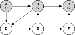
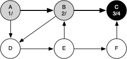
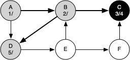
The following sequence of figures illustrates the depth-first search algorithm in action for a small graph. In these figures, the dotted lines indicate edges that are checked, but the node at the other end of the edge has already been added to the depth-first tree.
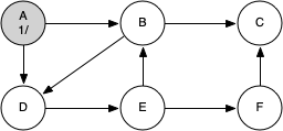
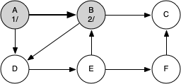
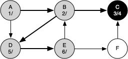
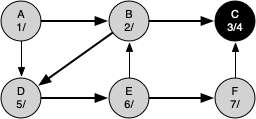
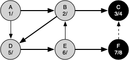
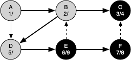
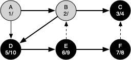
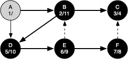
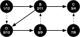
The search begins at vertex A of the graph. Since all of the vertices are white at the beginning of the search the algorithm visits vertex A. The first step in visiting a vertex is to set the color to gray, which indicates that the vertex is being explored, and the discovery time is set to 1. Since vertex A has two adjacent vertices (B, D) each of those need to be visited as well. We'll make the arbitrary decision that we will visit the adjacent vertices in alphabetical order.
Vertex B is visited next, so its color is set to gray and its discovery time is set to 2. Vertex B is also adjacent to two other nodes (C, D) so we will follow the alphabetical order and visit node C next.
Visiting vertex C brings us to the end of one branch of the tree. After coloring the node gray and setting its discovery time to 3, the algorithm also determines that there are no adjacent vertices to C. This means that we are done exploring node C and so we can color the vertex black and set the closing time to 4.
Since vertex C is the end of one branch, we now return to vertex B and continue exploring the nodes adjacent to B. The only additional vertex to explore from B is D, so we can now visit D and continue our search from vertex D. Vertex D quickly leads us to vertex E. Vertex E has two adjacent vertices, B and F. Normally we would explore these adjacent vertices alphabetically, but since B is already colored gray the algorithm recognizes that it should not visit B since doing so would put the algorithm in a loop! So exploration continues with the next vertex in the list, namely F.
Vertex F has only one adjacent vertex, C, but since C is colored black there is nothing else to explore, and the algorithm has reached the end of another branch. From here on, you will see the algorithm works its way back to the first node, setting closing times and coloring vertices black.
The discovery and closing times for each node display a property called the parenthesis property. This property means that all the children of a particular node in the depth-first tree have a later discovery time and an earlier closing time than their parent.
#include <iostream>
#include "pythonds3/cppds/graph_algos.hpp"   // DFSGraph (md listing above)
using namespace std;

int main() {
    DFSGraph g;
    g.addEdge("A", "B");  g.addEdge("B", "C");
    g.addEdge("A", "D");  g.addEdge("B", "D");
    g.addEdge("D", "E");  g.addEdge("E", "B");
    g.addEdge("E", "F");  g.addEdge("F", "C");
    g.dfs();
    printf("%4s|%9s|%8s|%9s\n", "Key", "Discover", "Closing", "Previous");
    for (auto& p : g.vertices)
        printf("%4s|%9d|%8d|%9s\n", p.first.c_str(),
               g.discovery[p.first], g.closing[p.first], p.second.previous.c_str());
    return 0;
}
Key| Discover| Closing| Previous
A| 1| 12|
B| 2| 11| A
C| 3| 4| B
D| 5| 10| B
E| 6| 9| D
F| 7| 8| E
Every vertex ends up black, with its discovery/closing times bracketing those of its descendants — the parenthesis property.
Iterating over the graph lists each directed edge exactly once, confirming the adjacency structure.
9.16. Depth First Search Analysis
The outer loops in dfs() take $O(|V|)$ excluding recursive edge scans: reset visits every vertex once, and the forest loop considers every vertex as a possible root once.
In dfsVisit(), adjacency scans total $O(|E|)$ because each directed adjacency entry is examined once from its source. Therefore DFS takes $O(|V|+|E|)$ time.
display_quiz(quiz_path+"bfs_dfs.json", max_width=800)
9.17. Topological Sorting
Course status: optional. Topological sorting is an official cppds section; this concise summary remains visible in RISE while the detailed derivation stays optional.
To demonstrate that computer scientists can turn just about anything into a graph problem, let’s consider the difficult problem of stirring up a batch of pancakes.
The recipe is really quite simple: 1 egg, 1 cup of pancake mix, 1 tablespoon oil, and $3 \over 4$ cup of milk. To make pancakes you must heat the griddle, mix all the ingredients together, and spoon the mix onto a hot griddle.
When the pancakes start to bubble you turn them over and let them cook until they are golden brown on the bottom. Before you eat your pancakes you are going to want to heat up some syrup.
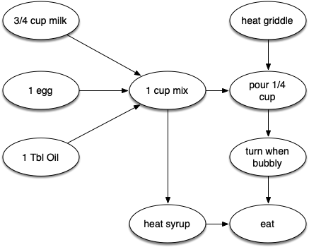
The difficult thing about making pancakes is knowing what to do first. As you can see, you might start by heating the griddle or by adding any of the ingredients to the pancake mix. To help us decide the precise order in which we should do each of the steps required to make our pancakes, we turn to a graph algorithm called the topological sort.
A topological sort takes a DAG and produces a linear ordering of all its vertices such that if the graph contains an edge $(v,w)$ then the vertex $v$ comes before the vertex $w$ in the ordering.
Directed acyclic graphs are used in many applications to indicate the precedence of events. Making pancakes is just one example; other examples include software project schedules, precedence charts for optimizing database queries, and multiplying matrices.
The topological sort is a simple but useful adaptation of a depth-first search. The algorithm for the topological sort is as follows:
- Call
g.dfs()for some graphg. The main reason we want to call depth-first search is to compute the closing times for each of the vertices.
Store the vertex keys in a
vector<string>ordered by decreasing closing time.Return that vector as the topological ordering.
Following shows the depth-first forest constructed by dfs on the pancake-making graph:
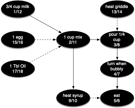
Figure below shows the results of applying the topological sort algorithm to our graph. Now all the ambiguity has been removed and we know exactly the order in which to perform the pancake-making steps.

9.18. Strongly Connected Components
Course status: optional. Strongly connected components are an official cppds section; this concise summary remains visible in RISE while the detailed derivation stays optional.
For the remainder of this chapter we turn to graphs formed by links between web pages and hosts on the internet.
Search engines like Google and Bing exploit the fact that the pages on the web form a very large directed graph. To transform the World Wide Web into a graph, we will treat a page as a vertex, and the hyperlinks on the page as edges connecting one vertex to another
You might make some interesting observations on these kind of graphs.You might conclude from this that there is some underlying structure to the Web that clusters together websites that are similar on some level.
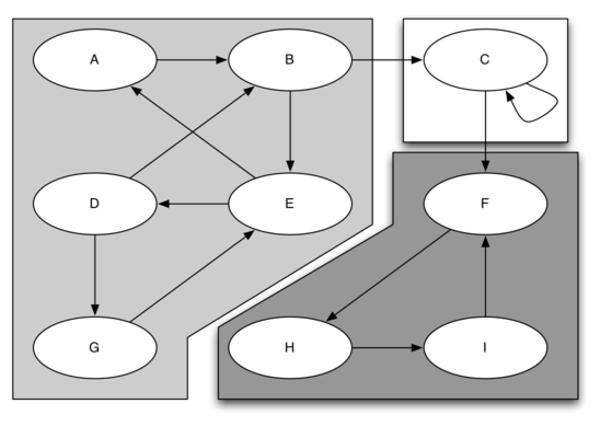
One graph algorithm that can help find clusters of highly interconnected vertices in a graph is called the strongly connected components algorithm, or SCC. We formally define a strongly connected component $C$ as the largest subset of vertices $C \subset V$ such that for every pair of vertices $v, w \in C$ we have a path from $v$ to $w$ and a path from $w$ to $v$.
Figure below shows a simple graph with three strongly connected components that are identified by the different shaded areas.
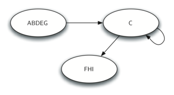
Once the strongly connected components have been identified, we can show a simplified view of the graph by combining all the vertices in one strongly connected component into a single larger vertex.
We will see that we can create a very powerful and efficient algorithm by making use of a depth-first search. Before we tackle the main SCC algorithm we must look at one other definition. The transposition of a graph is defined as the graph $G^T$ where all the edges in the graph have been reversed.
That is, if there is a directed edge from node A to node B in the original graph, then $G^T$ will contain an edge from node B to node A
We can now describe the algorithm to compute the strongly connected components for a graph:
Call
dfs()for the graph $G$ to compute the closing times for each vertex.Compute $G^T$.
Call
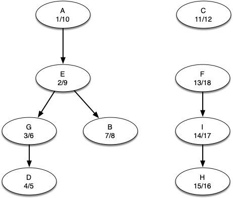
dfs()for the graph $G^T$ but in the main loop of DFS explore each vertex in decreasing order of closing time.Each tree in the forest computed in step 3 is a strongly connected component. Output the vertex IDs for each vertex in each tree in the forest to identify the component.
Let's trace the operation of the steps described above on the example graph above.
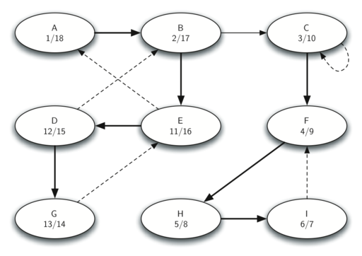
Below shows the starting and closing times computed for the original graph by the DFS algorithm.
Below shows the starting and closing times computed for the transposed graph by the DFS algorithm.
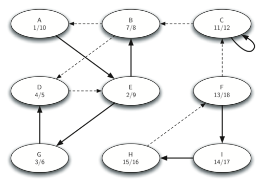
Finally, figure below shows the forest of three trees produced in step 3 of the strongly connected components algorithm.
9.19. Shortest Path Problems
When you surf the web, send an email, or log in to a laboratory computer from another location on campus, a lot of work is going on behind the scenes to get the information on your computer transferred to another computer. The in-depth study of how information flows from one computer to another over the internet is the primary topic for a class in computer networking.
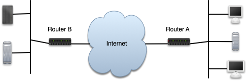
Figure above shows you a high-level overview of how communication on the internet works. When you use your browser to request a web page from a server, the request must travel over your local area network and out onto the internet through a router.
Each router on the internet is connected to one or more other routers. If you run the traceroute command at different times of the day, you are likely to see that your information flows through different routers at different times. This is because there is a cost associated with each connection between a pair of routers that depends on the volume of traffic, the time of day, and many other factors.
By this time it will not surprise you to learn that we can represent the network of routers as a graph with weighted edges.
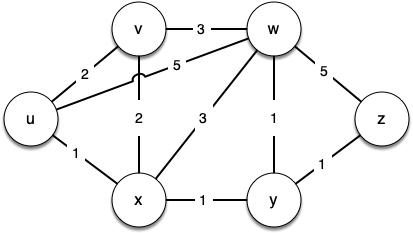
Figure below shows a small example of a weighted graph that represents the interconnection of routers in the internet. The problem that we want to solve is to find the shortest path, one with the smallest total weight along which to route any given message.
This problem should sound familiar because it is similar to the problem we solved using a breadth-first search, except that here we are concerned with the total weight of the path rather than the number of hops in the path. It should be noted that if all the weights are equal, the problem is the same!
display_quiz(quiz_path+"bfs.json", max_width=800)
9.20. Dijkstra's Algorithm
Dijkstra's algorithm is an iterative algorithm that provides us with the shortest path from one particular starting node to all other nodes in the graph. Again this is similar to the results of a breadth-first search.
To keep track of the total cost from the start node to each destination, we will make use of the distance instance variable in the Vertex class. The distance instance variable will contain the current total weight of the smallest weight path from the start to the vertex in question.
The algorithm iterates once for every vertex in the graph; however, the order that it iterates over the vertices is controlled by a priority queue. The value that is used to determine the order of the objects in the priority queue is distance.
A priority queue acts like a queue in that you dequeue an item by removing it from the front. However, in a priority queue the logical order of items inside a queue is determined by their priority. The highest priority items are at the front of the queue and the lowest priority items are at the back.
Thus when you enqueue an item on a priority queue, the new item may move all the way to the front.
When a vertex is first created, distance is set to a very large number. Theoretically you would set distance to infinity, but in practice we just set it to a number that is larger than any real distance we would have in the problem we are trying to solve.
In C++ we use the standard priority_queue as our min-heap: it stores (distance, key) pairs and, with greater<>, always pops the smallest distance first.
void dijkstra(Graph& g, string startKey) {
    // min-heap of (distance, vertex key) pairs
    priority_queue<pair<int, string>,
                   vector<pair<int, string>>,
                   greater<pair<int, string>>> pq;
    g.vertices[startKey].distance = 0;
    pq.push({0, startKey});

    while (!pq.empty()) {
        auto [distance, currentKey] = pq.top();
        pq.pop();
        if (distance > g.vertices[currentKey].distance) {
            continue;   // stale entry - an older candidate superseded by a better one
        }
        for (auto& n : g.vertices[currentKey].neighbors) {
            int newDistance = g.vertices[currentKey].distance + n.second;
            if (newDistance < g.vertices[n.first].distance) {
                g.vertices[n.first].distance = newDistance;
                g.vertices[n.first].previous = currentKey;
                pq.push({newDistance, n.first});
            }
        }
    }
}
Our C++ implementation uses a lazy priority queue. When relaxation improves a distance, it pushes a new (distance, key) pair instead of searching the heap for the old entry. When an older, larger entry reaches the top, the algorithm recognizes it as stale and skips it.
The priority queue can therefore contain more than one entry for a vertex. Every entry carries both the tentative distance and the vertex key, so popping the minimum entry still identifies which graph vertex to process.
After popping (queuedDistance, key), compare queuedDistance with the vertex's currently stored distance. If it is larger, a later relaxation has already superseded that entry; skip it without scanning the adjacency map.
There is no changePriority() call in this version. Each successful relaxation performs one heap push, so there are at most $O(|E|)$ pushed entries and the same number of pops.
Start at $u$ with distance = 0; every other vertex begins at INT_MAX (unreachable). Relaxing $u$'s incident edges assigns their first finite candidate distances and records $u$ as predecessor.
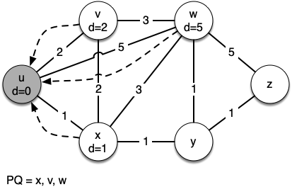
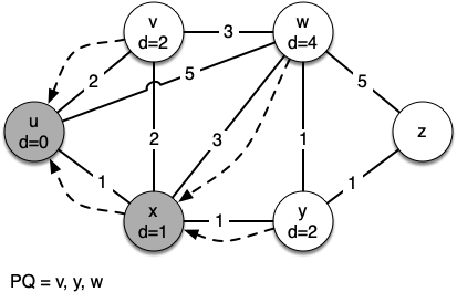
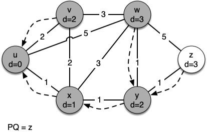
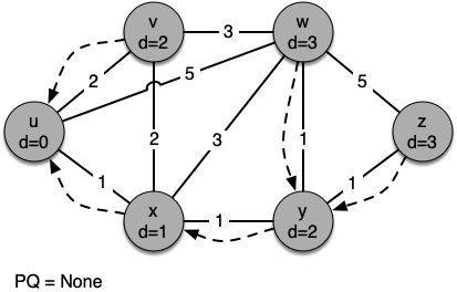
In the next iteration of the while loop we examine the vertices that are adjacent to $x$. The vertex $x$ is next because it has the lowest overall cost and therefore bubbled its way to the beginning of the priority queue. At $x$ we look at its neighbors $u,v,w$ and $y$.
When $x$ is popped, relaxation gives $y$ its first finite distance and improves the candidate for $w$. The lazy queue pushes the improved pairs; any superseded larger pair is skipped when it later reaches the top.
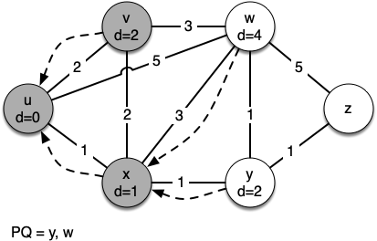
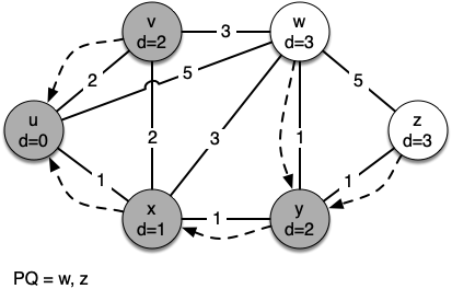
The next step is to look at the vertices neighboring $v$. This step results in no changes to the graph, so we move on to node $y$. At node $y$ we discover that it is cheaper to get to both $w$ and $z$, so we adjust the distances and predecessor links accordingly. Finally we check nodes $w$ and $z$. However, no additional changes are found and so the priority queue is empty and Dijkstra's algorithm exits.
#include <iostream>
#include "pythonds3/cppds/graph_algos.hpp"   // dijkstra (md listing above)
using namespace std;

int main() {
    Graph g;
    g.addEdge("u","v",2); g.addEdge("v","u",2); g.addEdge("v","w",3); g.addEdge("w","v",3);
    g.addEdge("w","z",5); g.addEdge("z","w",5); g.addEdge("u","x",1); g.addEdge("x","u",1);
    g.addEdge("u","w",5); g.addEdge("w","u",5); g.addEdge("x","v",2); g.addEdge("v","x",2);
    g.addEdge("x","w",3); g.addEdge("w","x",3); g.addEdge("x","y",1); g.addEdge("y","x",1);
    g.addEdge("y","w",1); g.addEdge("w","y",1); g.addEdge("y","z",1); g.addEdge("z","y",1);
    dijkstra(g, "u");
    for (auto& p : g.vertices)   // key: distance (previous)
        cout << p.first << ": " << p.second.distance
             << " (" << p.second.previous << ")" << endl;
    return 0;
}
u: 0 ()
v: 2 (u)
w: 3 (y)
x: 1 (u)
y: 2 (x)
z: 3 (y)
Every vertex now carries the length of the shortest path from u, and following previous pointers backwards reconstructs that path.
#include <iostream>
#include "pythonds3/cppds/graph_algos.hpp"   // dijkstra + findPath
using namespace std;

int main() {
    Graph g;
    g.addEdge("u","v",2); g.addEdge("v","u",2); g.addEdge("v","w",3); g.addEdge("w","v",3);
    g.addEdge("w","z",5); g.addEdge("z","w",5); g.addEdge("u","x",1); g.addEdge("x","u",1);
    g.addEdge("u","w",5); g.addEdge("w","u",5); g.addEdge("x","v",2); g.addEdge("v","x",2);
    g.addEdge("x","w",3); g.addEdge("w","x",3); g.addEdge("x","y",1); g.addEdge("y","x",1);
    g.addEdge("y","w",1); g.addEdge("w","y",1); g.addEdge("y","z",1); g.addEdge("z","y",1);
    dijkstra(g, "u");
    for (string v : findPath(g, "u", "z")) cout << v << " ";
    cout << endl;
    return 0;
}
u x y z
Dijkstra's correctness requires every edge weight to be non-negative; zero-weight edges are valid. A negative edge can reveal a shorter route after a vertex has been treated as final, so the greedy proof no longer applies. It does not imply that the program must loop forever: the result is simply not guaranteed. The course implementation rejects negative weights.
We will note that to route messages through the internet, other algorithms are used for finding the shortest path. One of the problems with using Dijkstra's algorithm on the internet is that you must have a complete representation of the graph in order for the algorithm to run. The implication of this is that every router has a complete map of all the routers in the internet!
In practice this is not the case and other variations of the algorithm allow each router to discover the graph as they go.
9.21. Analysis of Dijkstra's Algorithm
In the lazy C++ implementation, resetting all vertex distances costs $O(|V|)$ and only (0, start) is initially pushed. Scanning adjacency maps examines each directed edge once during the effective expansions.
Each successful relaxation adds one heap entry, so there are at most $O(|E|)$ pushes and pops. A heap operation costs $O(\log |E|)=O(\log |V|)$ for this simple map-backed graph, and ordered-map vertex lookup contributes the same logarithmic factor. The total is $O((|V|+|E|)\log |V|)$, with $O(|V|+|E|)$ storage including stale entries.
display_quiz(quiz_path+"dijk.json", max_width=800)
Exercise 1: Negative-edge precondition
The pictured graph contains negative-weight edges. What happens if it is passed to the course dijkstra(g, "A") implementation?
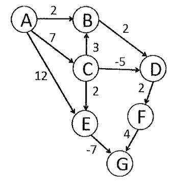
(A) It returns A->B->D.
(B) It returns A->C->D.
(C) It silently deletes the negative edges.
(D) It throws invalid_argument before running the priority-queue traversal.
Answer: (D). Lazy duplicate entries do not make Dijkstra valid for negative weights; the implementation explicitly enforces the non-negative precondition.
9.22. Prim's Spanning Tree Algorithm
For our last graph algorithm let's consider a problem that online game designers. The problem is that they want to efficiently transfer a piece of information to anyone and everyone who may be listening. This is important in gaming so that all the players know the very latest position of every other player!
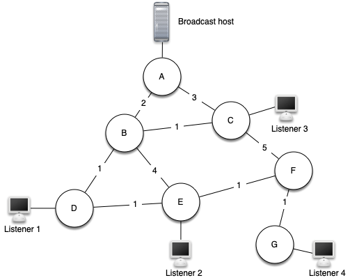
There are some brute force solutions to this problem. To begin, the broadcast host has some information that the listeners all need to receive. The simplest solution is for the broadcasting host to keep a list of all of the listeners and send individual messages to each.
In the above figure we show a small network with a broadcaster and some listeners. Using this first approach, four copies of every message would be sent. Assuming that the least cost path is used, let's see how many times each router would handle the same message.
All messages from the broadcaster go through router A, so A sees all four copies of every message. Router C sees only one copy of each message for its listener. However, routers B and D would see three copies of every message since routers B and D are on the cheapest path for listeners 1, 2, and 4! When you consider that the broadcast host must send hundreds of messages each second for a radio broadcast, that is a lot of extra traffic.
Another brute force solution is for the broadcast host to send a single copy of the broadcast message and let the routers sort things out. In this case, the easiest solution is a strategy called uncontrolled flooding:
Each message starts with a time to live (TTL) value set to some number greater than or equal to the number of edges between the broadcast host and its most distant listener. Each router gets a copy of the message and passes the message on to all of its neighboring routers. When the message is passed on the TTL is decreased. Because each router continues to send copies of the message to all its neighbors until the TTL value reaches 0, it is easy to convince yourself that uncontrolled flooding generates many more unnecessary messages than our first strategy.
The solution to this problem lies in the construction of a minimum weight spanning tree. Formally we define the minimum spanning tree $T$ for a graph $G = (V,E)$ as follows. $T$ is an acyclic subset of $E$ that connects all the vertices in $V$. The sum of the weights of the edges in $T$ is minimized.
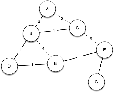
Below shows a simplified version of the broadcast graph and highlights the edges that form a minimum spanning tree for the graph.
Now to solve our broadcast problem, the broadcast host simply sends a single copy of the broadcast message into the network. Each router forwards the message to any neighbor that is part of the spanning tree, excluding the neighbor that just sent it the message.
In this example A forwards the message to B. B forwards the message to D and C. D forwards the message to E, which forwards it to F, which forwards it to G. No router sees more than one copy of any message, and all the listeners that are interested see a copy of the message.
Prim's algorithm is a greedy algorithm for a weighted undirected graph. At each step it chooses a safe edge: a minimum-weight edge crossing the cut between vertices already in the growing tree and vertices still outside it. The cheapest edge elsewhere in the graph is not necessarily eligible.
The course prim() requires one connected component containing every vertex. After the lazy priority queue empties, it compares the number of vertices added to the tree with g.vertices.size() and throws invalid_argument if the graph is disconnected.
While T is not yet a spanning tree
  Find an edge that is safe to add to the tree
  Add the new edge to T
The key step is to find a safe edge: among all edges crossing from the current tree to a vertex outside it, Prim's algorithm chooses one with minimum weight. Crossing the cut preserves connectivity without creating a cycle, and the cut property guarantees that this minimum-weight choice can belong to an MST.
void prim(Graph& g, string startKey) {
    priority_queue<pair<int, string>,
                   vector<pair<int, string>>,
                   greater<pair<int, string>>> pq;
    set<string> inTree;

    for (auto& p : g.vertices) {
        p.second.distance = INT_MAX;
        p.second.previous = "";
    }
    g.vertices[startKey].distance = 0;
    pq.push({0, startKey});
    ...
    ...
    while (!pq.empty()) {
        auto [distance, currentKey] = pq.top();
        pq.pop();
        if (inTree.count(currentKey)) continue;   // stale entry
        inTree.insert(currentKey);
        for (auto& n : g.vertices[currentKey].neighbors) {
            int newDistance = n.second;   // edge weight only, not path length!
            if (!inTree.count(n.first) && newDistance < g.vertices[n.first].distance) {
                g.vertices[n.first].distance = newDistance;
                g.vertices[n.first].previous = currentKey;
                pq.push({newDistance, n.first});
            }
        }
    }
    if (inTree.size() != g.vertices.size())
        throw invalid_argument("Prim requires a connected graph");
}
(complete listing: pythonds3/cppds/graph_algos.hpp)
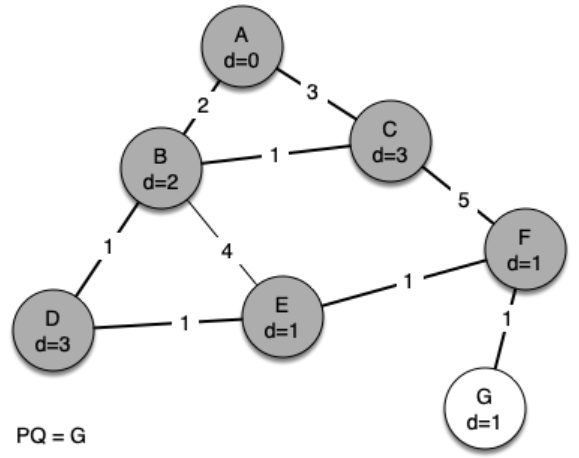
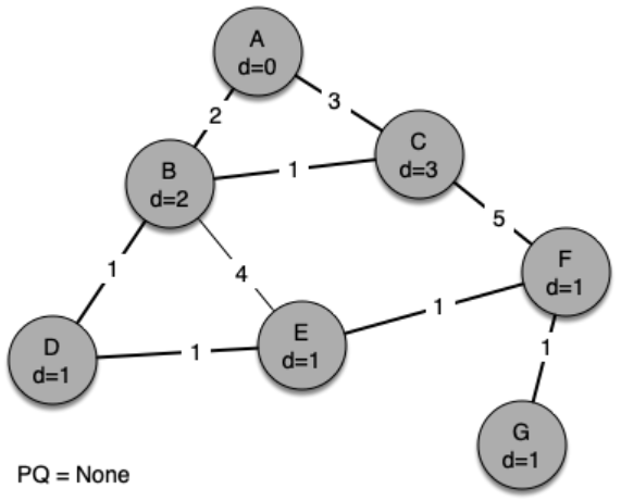
The following sequence of figures shows the algorithm in operation on our sample tree. We begin with the starting vertex as A. The distances to all the other vertices are initialized to infinity.
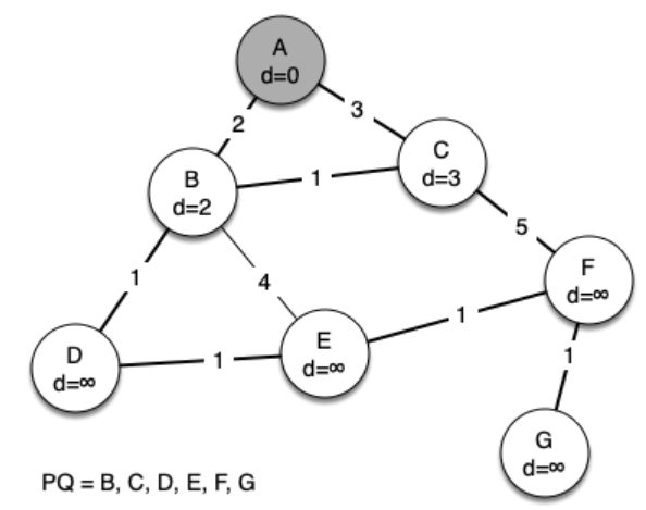
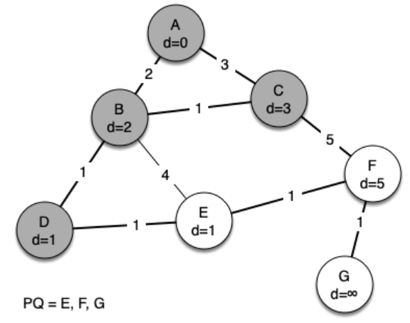
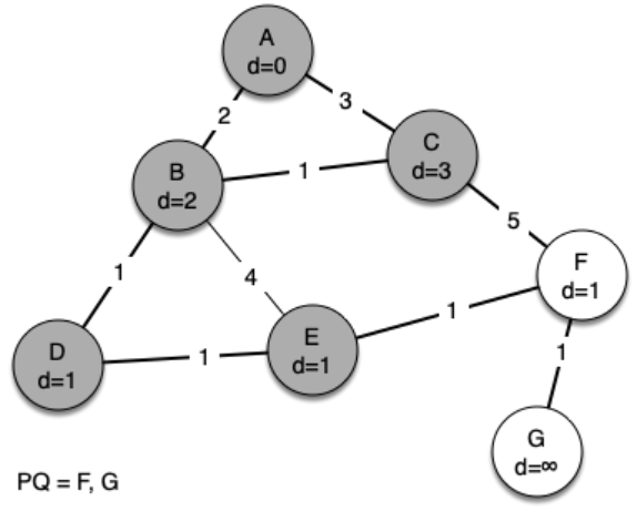
We begin with the starting vertex as A. The distances to all the other vertices are initialized to infinity. Looking at the neighbors of A we can update distances to two of the additional vertices, B and C, because the distances to B and C through A are less than infinite.
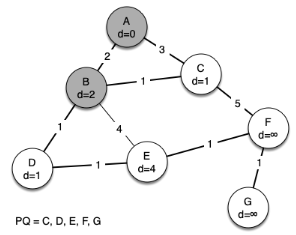
This moves B and C to the front of the priority queue. Update the predecessor links for B and C by setting them to point to A. It is important to note that we have not formally added B or C to the spanning tree yet. A node is not considered to be part of the spanning tree until it is removed from the priority queue.
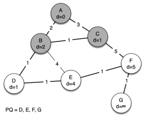
Since B has the smallest distance we look at B next. Examining B's neighbors we see that D and E can be updated. Both D and E get new distance values and their predecessor links are updated. Moving on to the next node in the priority queue we find C. The only node that C is adjacent to that is still in the priority queue is F; thus we can update the distance to F and adjust F’s position in the priority queue.
Now we examine the vertices adjacent to node D. We find that we can update E and reduce the distance to E from 4 to 1. When we do this we change the predecessor link on E to point back to D, thus preparing it to be grafted into the spanning tree but in a different location. The rest of the algorithm proceeds as you would expect, adding each new node to the tree.
#include <iostream>
#include "pythonds3/cppds/graph_algos.hpp"   // prim (md listing above)
using namespace std;

int main() {
    Graph g;
    g.addEdge("A","B",2); g.addEdge("B","A",2); g.addEdge("A","C",3); g.addEdge("C","A",3);
    g.addEdge("B","D",1); g.addEdge("D","B",1); g.addEdge("B","C",1); g.addEdge("C","B",1);
    g.addEdge("B","E",4); g.addEdge("E","B",4); g.addEdge("D","E",1); g.addEdge("E","D",1);
    g.addEdge("C","F",5); g.addEdge("F","C",5); g.addEdge("E","F",1); g.addEdge("F","E",1);
    g.addEdge("F","G",1); g.addEdge("G","F",1);

    prim(g, "A");
    cout << "MST edges: ";
    for (auto& p : g.vertices)
        if (p.second.previous != "")
            cout << "(" << p.second.previous << "," << p.first << ") ";
    cout << endl;
    return 0;
}
MST edges: (A,B) (B,C) (B,D) (D,E) (E,F) (F,G)
The printed edges form the minimum spanning tree rooted at A, discovered by repeatedly choosing the cheapest edge that crosses the current tree boundary.
display_quiz(quiz_path+"prim.json", max_width=800)
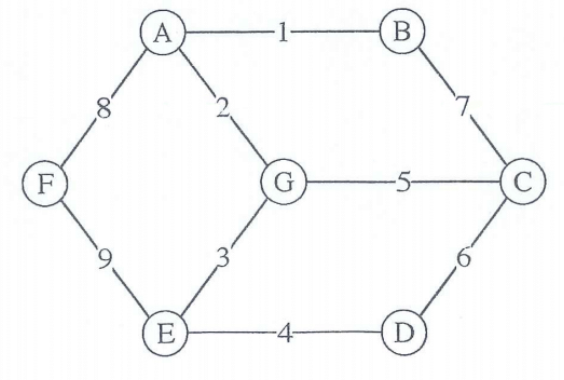
Exercise 2: Considering the following graph, when Prim's algorithm is used and starts from node F, what is the weight of the last edge to be added into the minimum spanning tree?
References
- Textbook: Problem Solving with Algorithms and Data Structures using C++ (cppds), Chapter 9 (Graphs and Graph Algorithms) — https://runestone.academy/ns/books/published/cppds/index.html
Key terms
Here's a brief definition for each of the key terms:
Graph: A data structure composed of a set of vertices (nodes) and edges (links) that connect pairs of these vertices. It is used to model relationships in complex systems.
Vertex: Also known as a node, it represents an entity within a graph and serves as the fundamental unit of the structure.
Edge: A connection between two vertices. In a directed graph, edges indicate a specific direction of relationship.
Weight: A numerical value assigned to an edge representing cost, distance, or another measure impacting traversal.
Path: A sequence of vertices connected by edges, defined by starting at one vertex and traversing through edges to reach another.
Cycle: A path that begins and ends at the same vertex, containing at least one edge and no repeated edges or internal vertices.
Acyclic Graph: A graph with no cycles, meaning it is impossible to return to a starting vertex by following edges.
Directed Graph: A graph where edges have a specific direction, indicating a one-way relationship from one vertex to another.
DAG (Directed Acyclic Graph): A directed graph containing no cycles, often used for task scheduling and sequences where tasks do not repeat.
Tree: A type of acyclic graph with a designated root vertex where all other vertices are connected by exactly one path to that root.
Adjacency Matrix: A square matrix used to represent a graph where elements indicate whether pairs of vertices are adjacent.
Adjacency List: A sparse representation storing only actual neighbors; this course uses ordered maps for vertices and neighbor weights.
Breadth-First Search (BFS): A search algorithm that explores all neighbor nodes at the current depth prior to moving on to nodes at the next depth level.
Knight's Tour: A sequence of moves on a chessboard where a knight visits every square exactly once.
Depth-First Search (DFS): A traversal algorithm that explores as far as possible along each branch before backtracking.
Search Tree: The tree formed by the predecessor (
previous) links that BFS or DFS records as it discovers vertices; following those links from any vertex leads back to the start.Heuristic: A technique designed to solve problems quickly or find approximate solutions when classic methods are too slow or infeasible.
Warnsdorff's Algorithm: A heuristic for the knight's tour where the knight always moves to the square with the fewest onward moves.
Depth-First Forest: A collection of trees formed during a depth-first search, where each tree corresponds to a set of vertices explored contiguously.
Parenthesis Property: A DFS property stating that discovery and finish time intervals for any two vertices are either entirely disjoint or nested.
Topological Sorting: A linear ordering of vertices in a directed graph where for every edge uv, vertex u comes before v.
Strongly Connected Components: Maximal subgraphs where every pair of vertices has a directed path to and from each other.
Shortest Path Problems: The challenge of finding a path between two vertices such that the sum of the weights of the edges is minimized.
Dijkstra's Algorithm: A single-source shortest-path algorithm for non-negative edge weights; the lazy C++ version pushes improved pairs and skips stale entries.
Priority Queue: A data structure where each element has a priority, and elements are served based on that priority rather than just arrival order.
Uncontrolled Flooding: A networking technique where a packet is sent to every outgoing link except the one it arrived on.
Minimum Spanning Tree (MST): A subset of edges connecting all vertices without cycles and with the minimum total edge weight.
Prim's Algorithm: An MST algorithm that repeatedly adds a minimum-weight edge crossing the cut from the current tree to an outside vertex.
Greedy Algorithms: A class of algorithms that build a solution by always choosing the next piece that offers the most immediate benefit.