Arrays

Execute the following two cells for the setup:

from jupyterquiz import display_quiz

path = "questions/ch3/"

1. Low-Level Arrays

2. Compact Array

3. Multidimensional Arrays (Matrix)

4. Sparse Martrix

A.1 Low-Level Arrays

In this section we will look at the principles behind low-level arrays. In C++ we get to work with the real thing: a C++ array is a contiguous block of memory — the very construct that Python's list is built on top of in its C implementation. Understanding it explains the performance of every sequence-based structure we will meet.

The key to Python's implementation of a list is to use a data type called an array common to C, C++, Java, and many other programming languages.

The array is very simple and is only capable of storing one kind of data. For example, you could have an array of integers or an array of floating point numbers, but you cannot mix the two in a single array.

The array only supports two operations: indexing and assignment to an array index.

The best way to think about an array is that it is one continuous block of bytes in the computer's memory. This block is divided up into $n$-byte chunks where $n$ is based on the data type that is stored in the array. Figure below illustrates the idea of an array that is sized to hold six floating point values.

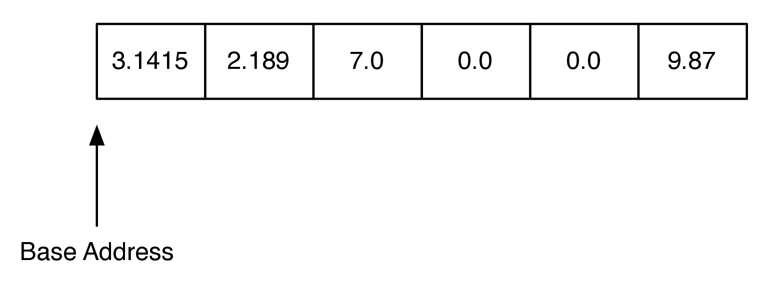
In C++, each double uses 8 bytes of memory, so an array of six doubles uses a total of 48 bytes. The base address is the location in memory where the array starts. The sizeof operator reports the size of any type or object:

using namespace std;
cout << sizeof(double) << " bytes per double" << endl;
cout << sizeof(int) << " bytes per int" << endl;
cout << sizeof(char) << " byte per char" << endl;

double data[6];
cout << sizeof(data) << " bytes for the whole array" << endl;
cout << &data[0] << " <- base address" << endl;
cout << &data[1] << " <- 8 bytes later" << endl;

8 bytes per double

4 bytes per int

1 byte per char

48 bytes for the whole array

0x7ffdf072de10 <- base address

0x7ffdf072de18 <- 8 bytes later

You have seen addresses before in Python for different objects that you have defined. For example: <__main__.Foo object at 0x5eca30> shows that the object Foo is stored at memory address 0x5eca30. The address is very important because an array implements the index operator using a very simple calculation:

item_address = base_address + index * size_of_object

For example, suppose that our array starts at location 0x000040, which is 64 in decimal. To calculate the location of the object at position 4 in the array we simply do the arithmetic:

$$64 + 4 \times 8$$

Clearly this kind of calculation is $O(1)$.

Of course this comes with some risks:

• First, since the size of an array is fixed, one cannot just add things on to the end of the array indefinitely without some serious consequences.

• Second, in some languages, like C, the bounds of the array are not even checked, so even though your array has only six elements in it, assigning a value to index 7 will not result in a runtime error!

display_quiz(path+"array1.json", max_width=800)

As you might imagine this can cause big problems that are hard to track down. In the Linux operating system, accessing a value that is beyond the boundaries of an array will often produce the rather uninformative error message "segmentation fault."

source:https://www.deviantart.com/froaproa/art/Programming-meme-983116183

The general strategy that a dynamic array (like C++'s vector or Python's list) uses is as follows:

• Allocate a raw array with extra capacity, and remember how many slots are actually used.
• When the array fills up, allocate a bigger raw array (typically twice the size), copy the elements over, and free the old one.
• Keep indexing O(1) by storing elements contiguously.

• Python uses a strategy called over-allocation to allocate an array with space for more objects than is needed initially.

When the initial array is finally filled up, a new, bigger array is over-allocated and the contents of the old array are copied to the new array!

Let's look at how the strategy outlined above works for a very simple implementation. To begin, we will only implement the constructor and the append(), size() and isEmpty() methods. We will call this class ArrayList.

In the constructor, we will need to initialize two instance variables. The first will keep track of the size of the current array; we will call this max_size. The second instance variable will keep track of the current end of the list; we will call this one last_index.

We will use a list to simulate an array:

class ArrayList {
    public:
        ArrayList(int initialCapacity = 8) {
            maxSize = initialCapacity;
            lastIndex = 0;
            myArray = new int[maxSize];
        }
        ~ArrayList() {
            delete[] myArray;
        }
    private:
        int maxSize;
        int lastIndex;
        int* myArray;   // raw dynamic array
};

void append(int val) {
    myArray[lastIndex] = val;
    lastIndex++;
}
int size() {
    return lastIndex;
}
bool isEmpty() {
    return lastIndex == 0;
}

Notice that the constructor method initializes the instance variables described above and then creates a zero element array called my_array.

Next, let us turn to the index operators. Below is our C++ implementation for indexing — we overload operator[] and check the bounds ourselves, throwing an exception on a bad index:

Even languages like C hide that calculation behind a nice array index operator, so in this case the C and the Python look very much the same:

int& operator[](int idx) {
    if (0 <= idx && idx < lastIndex) {
        return myArray[idx];
    }
    throw out_of_range("index out of bounds");
}

Returning a reference (int&) makes both reading a[i] and assigning a[i] = val work with a single operator — the compiler picks the right use automatically.

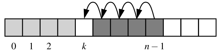
Finally, let's take a look at one of the more expensive list operations, insertion(). When we insert an item into an ArrayList we will need to first shift everything in the list at the insertion point and beyond ahead by one index position in order to make room for the item we are inserting. The process is illustrated in Figure below:

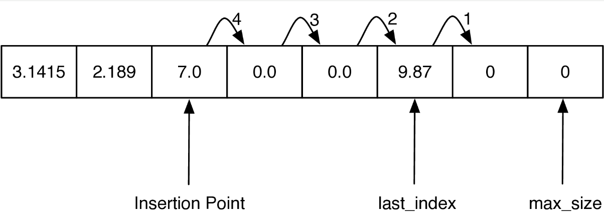
The key to implementing insert correctly is to realize that as you are shifting values in the array you do not want to overwrite any important data. The way to do this is to work from the end of the list back toward the insertion point, copying data forward.

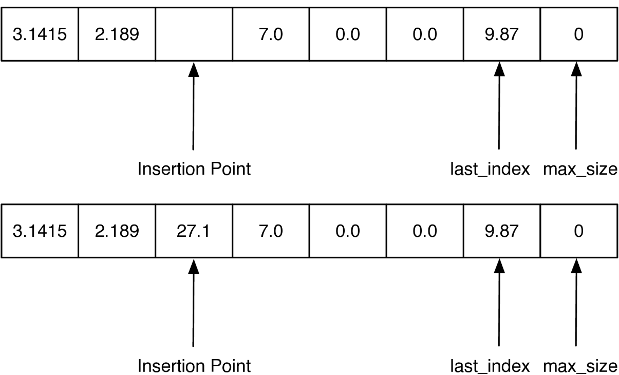
Our implementation of insert is shown below. Note how the range is set up on line to ensure that we are copying existing data into the unused part of the array first, and then subsequent values are copied over old values that have already been shifted.

void insert(int idx, int val) {
    for (int i = lastIndex; i > idx; i--) {
        myArray[i] = myArray[i - 1];
    }
    myArray[idx] = val;
    lastIndex++;
}

If the loop had started at the insertion point and copied that value to the next larger index position in the array, the old value would have been lost forever!

The performance of the insert is $O(n)$ since in the worst case we want to insert something at index 0 and we have to shift the entire array forward by one. On average we will only need to shift half of the array, but this is still $O(n)$.

The class offers another method, named remove(), that allows the caller to specify the value that should be removed (not the index at which it resides). Formally, it removes only the first occurrence of such a value from an array, or raises an error if no such value is found.

void remove(int val) {
    for (int i = 0; i < lastIndex; i++) {
        if (myArray[i] == val) {
            for (int j = i; j < lastIndex - 1; j++) {
                myArray[j] = myArray[j + 1];
            }
            lastIndex--;
            return;
        }
    }
    throw invalid_argument("value not found");
}

One part of the process searches from the beginning until finding the value at index k, while the rest iterates from k to the end in order to shift elements leftward. The complexity is again $O(n)$.

You can also implements other method like erase(idx).

The complete class (with erase(), growth handling, and printing) is collected in pythonds3/cppds/basic/. Here is the whole thing in action:

#include <iostream>
#include "dscpp/arraylist.hpp"   // the complete class of this section
using namespace std;

int main() {
    ArrayList myArray;
    myArray.append(31); myArray.append(77);
    myArray.append(17); myArray.append(93);
    myArray.display();
    cout << myArray[3] << " " << myArray.size() << endl;

    myArray.insert(3, 20);
    myArray.remove(31);
    myArray.display();

    myArray.erase(2);
    myArray[0] = 50;
    myArray.display();
    return 0;
}

31 77 17 93

93 4

77 17 20 93

50 17 93

display_quiz(path+"array2.json", max_width=800)

A.2 Compact Array

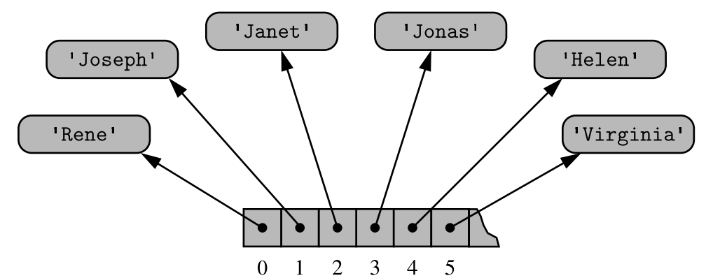
Assume that we have a collection of names such as {"Rene", "Joseph", "Janet", "Jonas", "Helen", "Virginia", ...}. In a referential layout the array cells hold pointers to string objects living elsewhere; each cell has the same fixed size no matter how long the name is.

To represent such a list with an array, Python must adhere to the requirement that each cell of the array use the same number of bytes. Yet the elements are strings, and strings naturally have different lengths!

Instead, Python represents a list or tuple instance using an internal storage mechanism of an array of object references. Although the relative size of the individual elements may vary, the number of bits used to store the memory address of each element is fixed (e.g., 64-bits per address). In this way, Python can support constant-time access!

On the other hand, strings are represented using an array of characters (not an array of references). We will refer to this more direct representation as a compact array because the array is storing the bits that represent the primary data (characters, in the case of strings)!

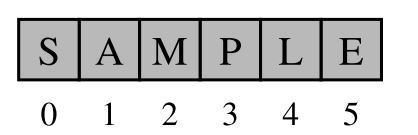
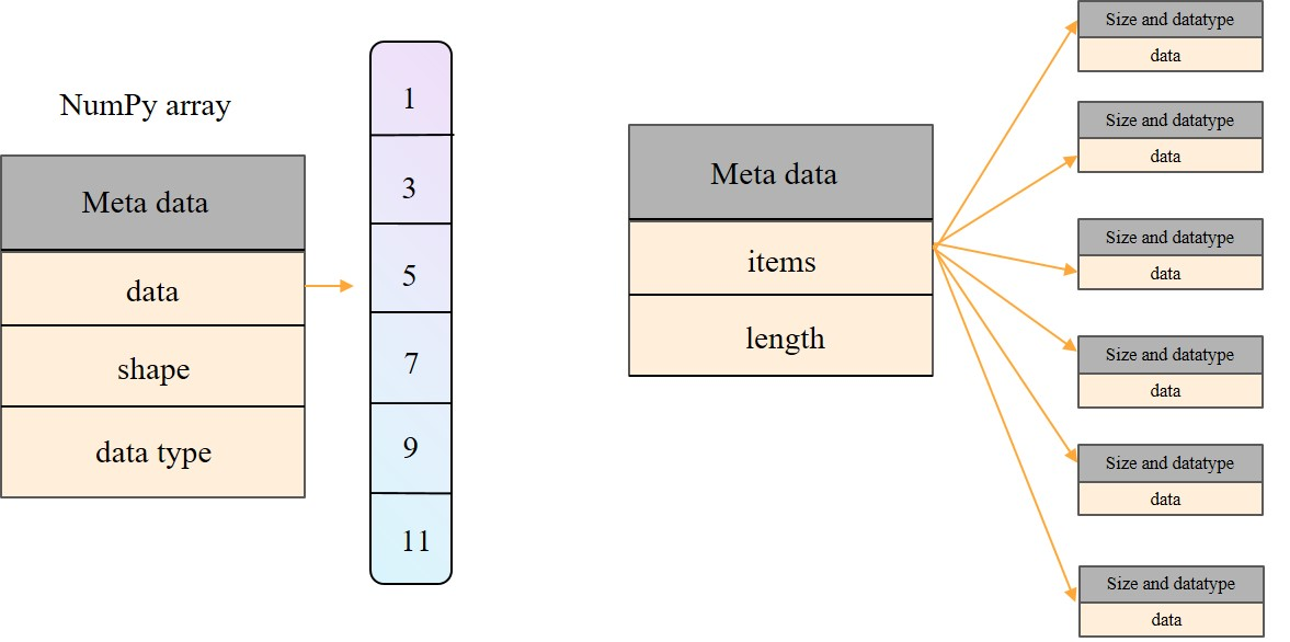
The overall memory usage will be much lower for a compact structure because there is no overhead devoted to the explicit storage of the sequence of memory references (in addition to the primary data)!

A referential structure will typically use 8 bytes (64 bits) for the memory address stored in the array, on top of whatever memory the object itself uses! In C++, an ordinary array is already compact: the element type determines exactly how many bytes each slot occupies.

using namespace std;
int primes[] = {2, 3, 5, 7, 11, 13, 17, 19};

cout << sizeof(primes[0]) << " bytes per element" << endl;
cout << sizeof(primes) << " bytes in total" << endl;
cout << sizeof(primes) / sizeof(primes[0]) << " elements" << endl;

string* names[3];   // a referential array: 3 pointers, 8 bytes each
cout << sizeof(names) << " bytes for three pointers" << endl;

4 bytes per element

32 bytes in total

8 elements

24 bytes for three pointers

The element type plays the role of NumPy's type code: declaring int (4 bytes) versus double (8 bytes) versus char (1 byte) tells the compiler precisely how many bits are needed per element of the array — no interpreter needed at run time.

Example 1: Try to compare the speed of increment an array of integers containing 0 to 9999 by 1 using python list and numpy array.

The type codes supported by the array module are formally based upon the native data types used by the C programming language. The precise number of bits for the C data types is system-dependent.

display_quiz(path+"array3.json", max_width=800)

A.3 Multidimensional Arrays

The arrays discussed so far are known as one-dimensional arrays because the data is organized linearly in only one direction. Many applications require that data be stored in more than one dimension. One common example is a table, which is an array that consists of rows and columns. This is commonly called a two-dimensional array (Matrix):

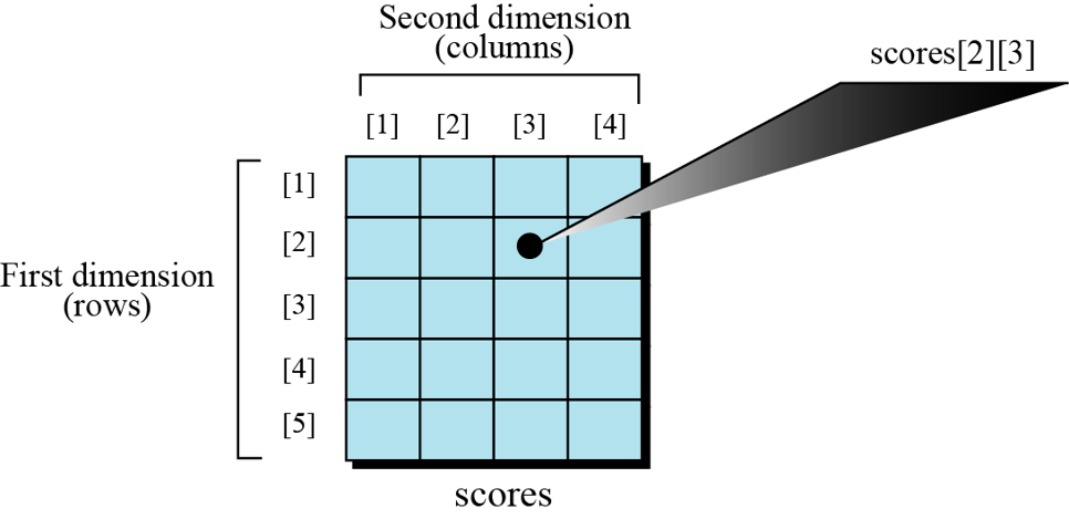
The array holds the scores of students in a class. There are five students in the class and each student has four different scores for four subjects. The variable scores[2][3] show the score of the second student in the third quiz.

Arranging the scores in a two-dimensional array can help us to find the average of scores for each student (the average over the row values) and find the average for each subject (the average over the column values) and so on. Note that multidimensional arrays — arrays with more than two dimensions — are also possible.

source: https://scipy-lectures.org/intro/numpy/operations.html

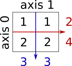
using namespace std;
// a matrix: initialize a 2D array with nested braces
int M[2][2] = {{1, 1}, {2, 2}};

cout << "M has " << sizeof(M) / sizeof(M[0]) << " rows and "
     << sizeof(M[0]) / sizeof(M[0][0]) << " columns, "
     << sizeof(M) << " bytes in total" << endl;

M has 2 rows and 2 columns, 16 bytes in total

Note the slicing of array works the same way as Python list!

using namespace std;
int M[2][2] = {{1, 1}, {2, 2}};
for (int j = 0; j < 2; j++) {
    cout << M[0][j] << " ";   // row 0
}
cout << endl;

1 1

using namespace std;
int M[2][2] = {{1, 1}, {2, 2}};
for (int i = 0; i < 2; i++) {
    cout << M[i][0] << " ";   // column 0
}
cout << endl;

1 2

using namespace std;
int M[2][2] = {{1, 1}, {2, 2}};
cout << M[1][1] << endl;   // row 1, column 1

2

A.3.1 Memory layout

The indexes in a one-dimensional array directly define the relative positions of the element in actual memory. A two-dimensional array, however, represents rows and columns. How each element is stored in memory depends on the computer!

Most computers use row-major storage, in which an entire row of an array is stored in memory before the next row. However, a computer may store the array using column-major storage, in which the entire column is stored before the next column. The following figure shows a two-dimensional array and how it is stored in memory using row-major or column-major storage. Row-major storage is more common.

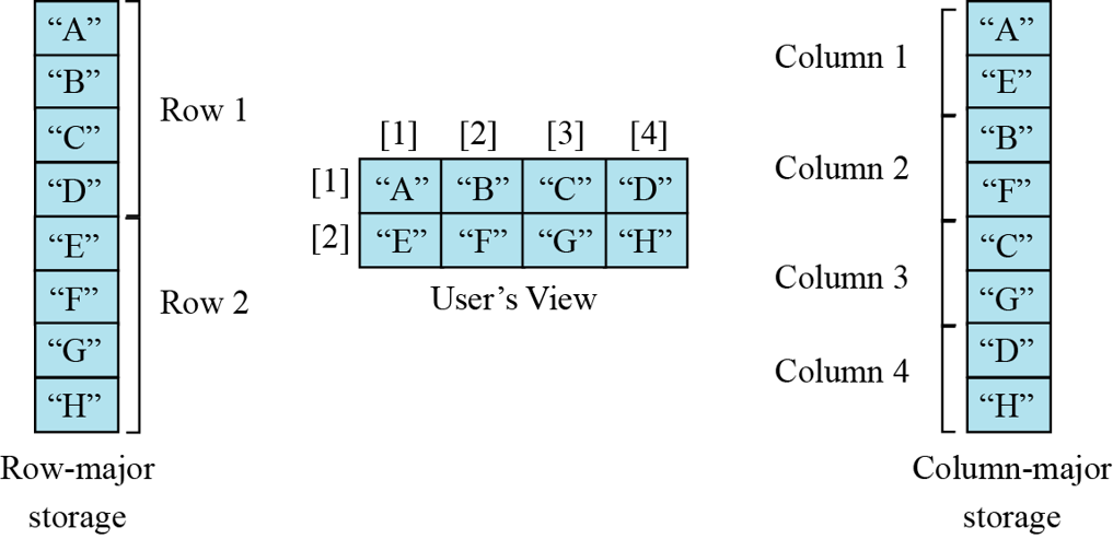
C++ two-dimensional arrays are row-major by definition — the language standard guarantees that M[0][0], M[0][1], M[1][0], M[1][1] sit consecutively in memory. We can see it directly by printing addresses:

using namespace std;
int M[2][2] = {{1, 1}, {2, 2}};
cout << &M[0][0] << " " << &M[0][1] << endl;   // 4 bytes apart
cout << &M[1][0] << " " << &M[1][1] << endl;   // next row follows immediately

0x7ffee0f64680 0x7ffee0f64684

0x7ffee0f64688 0x7ffee0f6468c

C++ has no built-in column-major layout (that is Fortran's convention). If an algorithm needs it, you store the matrix in a 1D array and do the index arithmetic yourself — note the formula swaps the roles of rows and columns:

using namespace std;
// column-major storage of a 2x2 matrix in a flat array
int flat[4];
int rows = 2, cols = 2;
int M[2][2] = {{1, 1}, {2, 2}};

for (int i = 0; i < rows; i++)
    for (int j = 0; j < cols; j++)
        flat[j * rows + i] = M[i][j];   // column-major: j*Rows + i

for (int k = 0; k < 4; k++) cout << flat[k] << " ";
cout << endl;

1 2 1 2

Exercise 1: We have stored the two-dimensional array students in the memory. The array is 100 × 4 (100 rows and 4 columns). Show the address of the element students[5][3] assuming that the element student[0][0] is stored in the memory location with address 0 and each element occupies only one memory location. The computer uses row-major storage.

using namespace std;
int student[100][4];
for (int i = 0; i < 100; i++)
    for (int j = 0; j < 4; j++)
        student[i][j] = i * 4 + j;   // fill with recognizable values

int* s = &student[0][0];   // view the 2D array as a flat 1D array
cout << student[5][3] << endl;

23

#include <cassert>
using namespace std;

int main() {
    int student[100][4];
    for (int i = 0; i < 100; i++)
        for (int j = 0; j < 4; j++) student[i][j] = i * 4 + j;
    int* s = &student[0][0];
    // Replace ? with your answer
    assert(student[5][3] == s[?]);
    cout << "Pass" << endl;
    return 0;
}

In file included from /usr/include/c++/13/cassert:44,
                 from /tmp/tmpikzgk11a.cpp:3:
/tmp/tmpikzgk11a.cpp: In function ‘int main()’:
/tmp/tmpikzgk11a.cpp:12:31: error: expected primary-expression before ‘?’ token
   12 |     assert(student[5][3] == s[?]);
      |                               ^
/tmp/tmpikzgk11a.cpp:12:32: error: expected primary-expression before ‘]’ token
   12 |     assert(student[5][3] == s[?]);
    ... (truncated; run the cell to see the full message)

We can use the following formula to find the location of an element, assuming each element occupies one memory location:

$y = x + Cols \times i + j$

where x defines the start address, Cols defines the number of columns in the array, i defines the row number of the element, j defines the column number of the element, and y is the address we are looking for!

display_quiz(path+"array4.json", max_width=800)

A.4 Sparse Martrix

A sparse matrix is a matrix that has a value of 0 for most elements. If the ratio of Number of Non-Zero (NNZ) elements to the size is less than 0.05, the matrix is sparse!

source: https://matteding.github.io/2019/04/25/sparse-matrices/

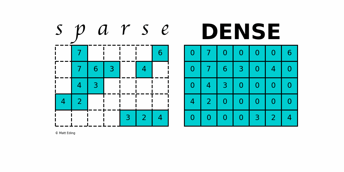
Storing information about all the 0 elements is inefficient, so we will assume unspecified elements to be 0. Using this scheme, sparse matrices can perform faster operations and use less memory than its corresponding dense matrix representation.

Different sparse formats have their strengths and weaknesses. A good starting point is looking at formats that are efficient for constructing these matrices. Typically you would start with one of these forms and then convert to another when ready to do calculations.

A.4.1 Coordinate Matrix

Perhaps the simplest sparse format to understand is the COOrdinate (COO) format. This variant uses three subarrays to store the element values and their coordinate positions.

source: https://matteding.github.io/2019/04/25/sparse-matrices/

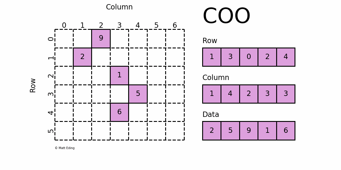
The savings on memory consumption is quite substantial as the matrix size increases. Managing data in a sparse structure is a fixed cost unlike the case for dense matrices.

The overhead incurred from needing to manage the subarrays is becomes negligible as data grows making it a great choice for some datasets!

A.4.2 Dictionary of Keys Matrix

Dictionary Of Keys (DOK) is very much like COO except that it uses a map with (row, column) pairs as keys to store coordinate-data information as key-value pairs. Using a hash-based container, identifying values at any given location has constant lookup time!

Use this format if you need the functionality that come with builtin dictionaries, but be mindful that hash tables hog more memory than arrays.

The SparseMatrix class uses a dictionary to store non-zero elements, with keys as (row, column) tuples and values as the non-zero elements.

class SparseMatrix {
    public:
        SparseMatrix() {}

        // read access: return the stored value, or 0 for unset positions
        double operator()(size_t i, size_t j) const {
            auto it = data.find({i, j});
            if (it != data.end()) {
                return it->second;
            }
            return 0.0;
        }
    private:
        map<pair<size_t, size_t>, double> data;
};

// write access: inserts the position if absent
double& operator()(size_t i, size_t j) {
    return data[{i, j}];
}

size_t nnz() const {
    return data.size();   // number of non-zeros
}

We can easily implement relational operations as follows:

bool operator==(const SparseMatrix& other) const {
    return data == other.data;
}

bool operator!=(const SparseMatrix& other) const {
    return !(*this == other);
}

// how sparse is the matrix, given its logical dimensions?
double sparsity(size_t rows, size_t cols) const {
    return 1.0 - double(data.size()) / double(rows * cols);
}

The arithmetic operation is slightly more involved — every coordinate present in either operand must appear in the result:

SparseMatrix operator+(const SparseMatrix& other) const {
    SparseMatrix result;
    for (const auto& item : data) {
        result.data[item.first] = item.second + other(item.first.first, item.first.second);
    }
    for (const auto& item : other.data) {
        if (data.find(item.first) == data.end()) {
            result.data[item.first] = item.second;
        }
    }
    return result;
}

Multiplication only needs to visit the non-zero entries of both operands — this is where the sparse representation really pays off:

SparseMatrix operator*(const SparseMatrix& other) const {
    SparseMatrix result;
    for (const auto& item1 : data) {
        for (const auto& item2 : other.data) {
            if (item1.first.second == item2.first.first) {
                result(item1.first.first, item2.first.second)
                    += item1.second * item2.second;
            }
        }
    }
    return result;
}

The conversion from dense matrix can be written as follows:

void fromDenseMatrix(const vector<vector<double>>& matrix) {
    for (size_t i = 0; i < matrix.size(); ++i) {
        for (size_t j = 0; j < matrix[i].size(); ++j) {
            if (matrix[i][j] != 0) {
                data[{i, j}] = matrix[i][j];
            }
        }
    }
}

We can play the class as follows:

The complete class lives in pythonds3/cppds/basic/sparse.cpp. Here it is in action:

#include <iostream>
#include "dscpp/sparsematrix.hpp"
using namespace std;

int main() {
    vector<vector<double>> denseMatrix = {{1, 0, 0}, {0, 2, 0}, {0, 0, 3}};
    SparseMatrix sparseMatrix;
    sparseMatrix.fromDenseMatrix(denseMatrix);
    cout << sparseMatrix << endl;

    SparseMatrix matrix1({{{0, 1}, 1}, {{1, 1}, 2}, {{2, 2}, 3}});
    SparseMatrix matrix2({{{1, 1}, 3}, {{2, 2}, 4}});

    cout << matrix1 + matrix2 << endl;
    cout << matrix1 - matrix2 << endl;
    cout << matrix1 * matrix2 << endl;
    return 0;
}

(0, 0):

1 (1, 1): 2 (2, 2): 3

(0, 1): 1 (1, 1): 5 (2, 2): 7

(0, 1): 1 (1, 1): -1 (2, 2): -1

(0, 1): 3 (1, 1): 6 (2, 2): 12

Each printed line lists the non-zero entries as (row, column): value pairs — everything absent is an implicit zero.

display_quiz(path+"array5.json", max_width=800)

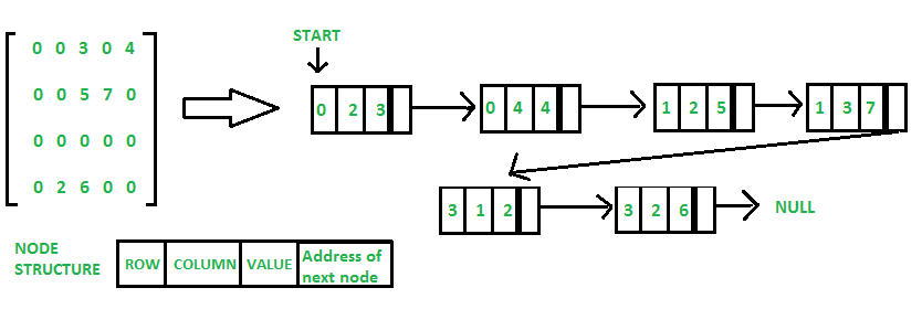
A.4.3 Linear list

source: https://www.geeksforgeeks.org/sparse-matrix-representation/

from jupytercards import display_flashcards
fpath = "flashcards/"
display_flashcards(fpath + 'ch3.json')

References

1. Textbook: Problem Solving with Algorithms and Data Structures using C++ (cppds) — https://runestone.academy/ns/books/published/cppds/index.html
2. Forouzan, Foundations of Computer Science, Ch 11 (Data Organization)

Key terms

Here's a brief definition for each of the key terms:

• Array: A data structure consisting of a collection of elements, each identified by at least one array index or key. Arrays store elements of the same data type and allocate memory in a contiguous block.

• Segmentation Fault: An error that occurs when a program attempts to access memory that it is not allowed to, often leading to a program crash. This can happen for reasons like accessing an array beyond its bounds.

• Referential Array: An array that contains references (or pointers) to objects rather than the objects themselves. This allows for more flexible data structures, such as linked lists or trees, to be built using arrays.

• Compact Array: An array with minimal memory overhead, designed to store data densely without pointers or references. It usually implies that the array is precisely as large as necessary to hold its contents.

• Multidimensional Array: An array containing one or more arrays. The data is organized in a grid or matrix, accessible through multiple indices. For example, a two-dimensional array represents rows and columns.

• Column Major: A method of storing multidimensional arrays in memory where elements are stored column by column. This contrasts with row-major order, affecting how operations like traversals and computations are optimized.

• Row Major: A method of storing multidimensional arrays in memory where elements are stored row by row. This is the default storage method in many programming languages, affecting the efficiency of various operations.

• Sparse Matrix: A matrix in which most of the elements are zero. Storing only the non-zero elements in memory-efficient data structures saves space and computational resources.

• Coordinate Format (COO): A method for storing sparse matrices by representing them as three lists (row, column, value), where each list represents a non-zero element and its position in the matrix.

• Dictionaries of Keys Matrix (DOK): A sparse matrix representation using a hash map (such as std::map or std::unordered_map) where each key is a (row, column) pair and the value is the element value.

• Sparse Matrix as Linear List: Representing a sparse matrix by linking the non-zero elements together in a linear list, possibly sorted by row and column indices. This approach can optimize certain operations but may be less efficient for random access compared to other sparse matrix representations.