Algorithm Analysis

1. What Is Algorithm Analysis?

2. Big O Notation

3. Example: Anagram Detection

4. Benchmark of C++ Data Structures: Vectors/Maps

2.1~2.2 What Is Algorithm Analysis?

An interesting question often arises. When two programs solve the same problem but look different, is one program better than the other?

In order to answer this question, we need to remember that there is an important difference between a program and the underlying algorithm that the program is representing!

There may be many programs for the same algorithm, depending on the programmer and the programming language being used!

To explore this difference further, consider the function that computes the sum of the first $n$ integers. The algorithm uses the idea of an accumulator variable that is initialized to 0. The solution then iterates through the $n$ integers, adding each to the accumulator.

#include <iostream>
using namespace std;

long long sumOfN(long long n) {
    long long theSum = 0;
    for (long long i = 1; i <= n; i++) {
        theSum = theSum + i;
    }
    return theSum;
}

int main() {
    cout << sumOfN(10) << endl;
    return 0;
}

55

Now look at the function below:

#include <iostream>
using namespace std;

long long foo(long long tom) {
    long long fred = 0;
    for (long long bill = 1; bill <= tom; bill++) {
        long long barney = bill;
        fred = fred + barney;
    }
    return fred;
}

int main() {
    cout << foo(10) << endl;
    return 0;
}

55

At first glance it may look strange, but this function is essentially doing the same thing as the previous one. Here, we did not use good identifiers for readability, and we used an extra assignment statement that was not really necessary!

The function sumOfN() is certainly better than the function foo() if you are concerned with readability. Easy to read and easy to understand is important for beginner. In this course, however, we are also interested in characterizing the algorithm itself.

Algorithm analysis is concerned with comparing algorithms based upon the amount of computing resources that each algorithm uses.

We want to be able to consider two algorithms and say that one is better than the other because it is more efficient in its use of those resources or perhaps because it simply uses fewer.

There are two different ways to look at this. One way is to consider the amount of space or memory an algorithm requires to solve the problem.

As an alternative to space requirements, we can analyze and compare algorithms based on the amount of time they require to execute.

One way is that we can measure the execution time for the function sumOfN() to do a benchmark analysis. In C++, we can benchmark a function by noting the starting time and ending time within the system we are using.

#include <iostream>
#include <chrono>
using namespace std;
using namespace std::chrono;

long long sumOfN2(long long n, double& seconds) {
    auto start = steady_clock::now();
    long long theSum = 0;
    for (long long i = 1; i <= n; i++) theSum = theSum + i;
    seconds = duration<double>(steady_clock::now() - start).count();
    return theSum;}
int main() {
    for (int run = 0; run < 3; run++) {
        double secs;
        long long s = sumOfN2(10, secs);
        cout << "Sum is " << s  << " required " << fixed << setprecision(7)  << setw(10) << secs  << " seconds" << endl;}
    return 0;
}

Sum is 55 required  0.0000001 seconds
Sum is 55 required  0.0000001 seconds
Sum is 55 required  0.0000000 seconds

We discover that the time is fairly consistent. What if we run the function adding the first 1,000,000 integers?

#include <iostream>
#include <chrono>

using namespace std;
using namespace std::chrono;

long long sumOfN2(long long n, double& seconds) {
    auto start = steady_clock::now();
    long long theSum = 0;
    for (long long i = 1; i <= n; i++) theSum = theSum + i;
    seconds = duration<double>(steady_clock::now() - start).count();
    return theSum;}
int main() {
    for (int run = 0; run < 3; run++) {
        double secs;
        long long s = sumOfN2(1'000'000, secs);
        cout << "Sum is " << s  << " required " << fixed << setprecision(7)  << setw(10) << secs  << " seconds" << endl;}
    return 0;
}

Sum is 500000500000 required  0.0015442 seconds
Sum is 500000500000 required  0.0015267 seconds
Sum is 500000500000 required  0.0015342 seconds

Now consider the following function, which shows a different means of solving the summation problem. This function takes advantage of a closed equation $\sum_{i=1}^{n} i = \frac {(n)(n+1)}{2}$ to compute the sum of the first $n$ integers without iterating.

#include <iostream>
#include <chrono>
using namespace std;
using namespace std::chrono;

long long sumOfN3(long long n, double& seconds) {
    auto start = steady_clock::now();
    long long theSum = (n * (n + 1)) / 2;
    seconds = duration<double>(steady_clock::now() - start).count();
    return theSum;}
int main() {
    for (int run = 0; run < 3; run++) {
        double secs;
        long long s = sumOfN3(10, secs);
        cout << "Sum is " << s  << " required " << fixed << setprecision(7)  << setw(10) << secs  << " seconds" << endl;}
    return 0;
}

Sum is 55 required  0.0000001 seconds
Sum is 55 required  0.0000000 seconds
Sum is 55 required  0.0000000 seconds

If we do the same benchmark measurement for sum_of_n_3(), using four different values for $n$ (100,000, 1,000,000, 10,000,000, and 100,000,000), we get the following results:

#include <iostream>
#include <chrono>
using namespace std; using namespace std::chrono;
long long sumOfN3(long long n, double& seconds) {
    auto start = steady_clock::now();
    long long theSum = (n * (n + 1)) / 2;
    seconds = duration<double>(steady_clock::now() - start).count();
    return theSum;}
int main() {
    long long ns[] = {100'000, 1'000'000, 10'000'000, 100'000'000};
    for (long long n : ns) {
        double secs;
        long long s = sumOfN3(n, secs);
        cout << "Sum is " << s  << " required " << fixed << setprecision(7)  << setw(10) << secs  << " seconds" << endl;
    }
}

Sum is 5000050000 required  0.0000000 seconds
Sum is 500000500000 required  0.0000001 seconds
Sum is 50000005000000 required  0.0000001 seconds
Sum is 5000000050000000 required  0.0000000 seconds

First, the times recorded above are shorter than any of the previous examples. Second, they are very consistent no matter what the value of $n$. It appears that sum_of_n_3() is hardly impacted by the number of integers being added.

Intuitively, we can see that the iterative solutions seem to be doing more work since some program steps are being repeated. Also, the time required for the iterative solution seems to increase as we increase the value of $n$.

However, if we ran the same function on a different computer or used a different programming language, we would likely get different results. It could take even longer to perform sumOfN3() if the computer were older.

We need a better way to characterize these algorithms with respect to execution time. The benchmark does not really provide us with a useful measurement because it is dependent on a particular machine, program, time of day, compiler, and programming language.

We would like to have a characterization that is independent of the program or computer being used. This measure would then be useful for judging the algorithm alone and could be used to compare algorithms across implementations!

2.3 Big O Notation

If each of these steps is considered to be a basic unit of computation, then the execution time for an algorithm can be expressed as the number of steps required to solve the problem!

Deciding on an appropriate basic unit of computation can be a complicated problem and will depend on how the algorithm is implemented.

A good basic unit of computation for comparing the summation algorithms might be the number of assignment statements performed to compute the sum.

In the function sumOfN():

long long sumOfN(long long n) {
    long long theSum = 0;
    for (long long i = 1; i <= n; i++) {
        theSum = theSum + i;
    }
    return theSum;
}

The number of assignment statements is 1 (the_sum = 0) plus the value of $n$ (the number of times we perform the_sum = the_sum + 1). We can denote this by a function, call it $T$, where $T(n)= n+1$.

The parameter $n$ is often referred to as the size of the problem, and we can read this as $T(n)$ is the time it takes to solve a problem of size $n$, namely $n+1$ steps.

We can then say that the sum of the first 100,000 integers is a bigger instance of the summation problem than the sum of the first 1,000. Our goal then is to show how the algorithm's execution time (steps) changes with respect to the size of the problem.

It turns out that the exact number of operations is not as important as determining the most dominant part of the function. In other words, as the problem gets larger, some portion of the function tends to overpower the rest.

The order of the magnitude of the function describes the part of $T(n)$ that increases the fastest as the value of $n$ increases. Order of magnitude is often called Big O notation (for order) and written as $O(f(n))$.

It provides a useful approximation of the actual number of steps in the computation. The function $f(n)$ provides a simple representation of the dominant part of the original $T(n)$.

In the above example, $T(n)=n+1$. As $n$ gets larger, the constant 1 will become less and less significant to the final result. If we are looking for an approximation for $T(n)$, then we can drop the 1 and simply say that the running time is $O(n)$.

It is important to note that the 1 is certainly significant for $T(n)$. However, as $n$ gets large, our approximation will be just as accurate without it.

As another example, suppose that for some algorithm, the exact number of steps is $T(n)=5n^2+27n+1005$. When $n$ is small, say 1 or 2, the constant 1005 seems to be the dominant part of the function. However, as $n$ gets larger, the $n^2$ term becomes the most important! .

In fact, when $n$ is really large, the other two terms become insignificant for the final result. Again, to approximate $T(n)$ as $n$ gets large, we can ignore the other terms and focus on $5n^2$.

In addition, the coefficient $5$ becomes insignificant as $n$ gets large. We would say then that the function $T(n)$ has an order of magnitude $f(n)=n^2$, or simply that it is $O(n^2)$.

Sometimes the performance of an algorithm depends on the exact values of the data rather than simply the size of the problem. For these kinds of algorithms we need to characterize their performance in terms of best-case, worst-case, or average-case performance.

The worst-case performance refers to a particular data set where the algorithm performs especially poorly, whereas a different data set for the exact same algorithm might have extraordinarily good (best-case) performance.

However, in most cases the algorithm performs somewhere in between these two extremes (average-case performance).

A number of very common order of magnitude functions will come up over and over as you study algorithms:

f(n)	Name
1	Constant
log(n)	Logarithmic
n	Linear
n log(n)	Log linear
n2	Quadratic
n3	Cubic
2n	Exponential

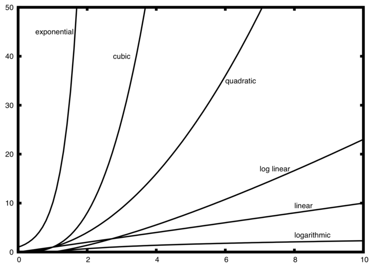
Notice that when $n$ is small, the functions are not very well defined with respect to one another. It is hard to tell which is dominant.

As a final example, suppose that we have the fragment of C++ code:

using namespace std;
int n = 100;
// Start of the code
int a = 5;
int b = 6;
int c = 10;
for (int i = 0; i < n; i++) {
    for (int j = 0; j < n; j++) {
        int x = i * i;
        int y = j * j;
        int z = i * j;
    }
}
for (int k = 0; k < n; k++) {
    int w = a * k + 45;
    int v = b * b;
}
int d = 33;

• The first part is the constant 3, representing the three assignment statements at the start of the fragment.
• The second part is $3n^2$ due to the nested iteration.
• The third part is $2n$ and the fourth part is the constant 1, representing the final assignment statement.

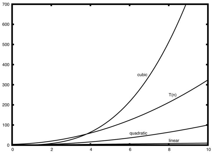
This gives us $T(n)=3+3n^2+2n+1=3n^2+2n+4$. We can see that the $n^2$ term will be dominant and therefore this code is $O(n^2)$. All of the other terms as well as the coefficient on the dominant term can be ignored as $n$ grows larger!

display_quiz(path+"BigO1.json", max_width=800)

display_quiz(path+"BigO2.json", max_width=800)

display_quiz(path+"BigO3.json", max_width=800)

2.4 An Anagram Detection Example

A good example problem for showing algorithms with different orders of magnitude is the classic anagram detection problem for strings. One string is an anagram of another if the second is simply a rearrangement of the first. For example, "heart" and "earth" are anagrams. The strings "python" and "typhon" are anagrams as well!

For the sake of simplicity, we will assume that the two strings in question are of equal length and that they are made up of symbols from the set of 26 lowercase alphabetic characters.

Our goal is to write a boolean function that will take two strings and return whether they are anagrams.

2.4.1 Solution 1: Anagram Detection Checking Off

Our first solution to the anagram problem will:

1. Check the lengths of the strings

2. Check to see that each character in the first string actually occurs in the second. If it is possible to check off each character, then the two strings must be anagrams.

To determine whether the two strings are anagrams, we compare each character in s1 with the remaining characters from s2. We first copy the characters of s2 into a vector<char> called aList. Whenever a matching character is found, it is removed from aList, so that the same character cannot be matched again. If every character in s1 can be matched and removed, the two strings are anagrams.

bool anagramSolution1(string s1, string s2) {
    bool stillOK = true;
    if (s1.length() != s2.length()) stillOK = false;   // Step 1
    vector<char> aList(s2.begin(), s2.end());
    unsigned pos1 = 0;
    while (pos1 < s1.length() && stillOK) {            // Step 2
        unsigned pos2 = 0;
        bool found = false;
        while (pos2 < aList.size() && !found) {
            if (s1[pos1] == aList[pos2]) found = true;
            else pos2 = pos2 + 1;
        }
        ...

(complete listing: https://github.com/phonchi/pythonds3/blob/master/cppds/anagram.hpp)

#include <iostream>
#include "pythonds3/cppds/anagram.hpp"
using namespace std;

int main() {
    cout << boolalpha << anagramSolution1("apple", "pleap") << endl;
    return 0;
}

true

Expected output: true — every character of s1 was checked off in s2.

Each of the $n$ characters in s1 will cause an iteration through up to $n$ characters in the list from s2. Each of the $n$ positions in the list will be visited once to match a character from s1. The number of visits then becomes the sum of the integers from 1 to $n$. Therfore, $\sum_{i=1}^{n} i = \frac {n(n+1)}{2}$!

As $n$ gets large, the $n^2$ term will dominate. Therefore, this solution is $O(n^2)$.

2.4.2 Solution 2: Sort and Compare

Another solution to the anagram problem will make use of the fact that even though s1 and s2 are different, they are anagrams only if they consist of exactly the same characters.

So if we begin by sorting each string alphabetically from a to z, we will end up with the same string if the original two strings are anagrams!

#include <iostream>
#include <string>
#include <algorithm>
using namespace std;

bool anagramSolution2(string s1, string s2) {
    sort(s1.begin(), s1.end());
    sort(s2.begin(), s2.end());
    unsigned pos = 0;
    bool matches = true;
    while (pos < s1.length() && matches) {
        if (s1[pos] == s2[pos]) pos = pos + 1;
        else matches = false;
    }
    return matches;
}

int main() {
    cout << boolalpha << anagramSolution2("apple", "pleap") << endl;
    return 0;
}

true

Expected output: true — after sorting, both strings become aelpp.

At first glance you may be tempted to think that this algorithm is $O(n)$, since there is one simple iteration to compare the $n$ characters after the sorting process. However, the two calls to the C++ sort() method are not without their own cost. As we will see in Chapter 7, sorting is typically either $O(n^2)$ or $O(n\log n)$, so the sorting operations dominate the iteration.

2.4.3 Solution 3: Brute Force

A brute force technique for solving a problem tries to exhaust all possibilities. For the anagram detection problem, we can simply generate a list of all possible strings using the characters from s1 and then see if s2 occurs.

However, when generating all possible strings from s1, there are $n$ possible first characters, $n-1$ possible characters for the second position, and so on. The total number of candidate strings is $n!$. Although some of the strings may be duplicates, the program cannot know this ahead of time!

It turns out that $n!$ grows even faster than $2^n$ as $n$ gets large. In fact, if s1 were 20 characters long, there would be $20! = 2,432,902,008,176,640,000$ possible candidate strings. If we processed one possibility every second, it would still take us $77,146,816,596$ years to go through the entire vector!

2.4.4 Solution 4: Count and Compare

Our final solution to the anagram problem takes advantage of the fact that any two anagrams will have the same number of a's, the same number of b's, the same number of c's, and so on.

In order to decide whether two strings are anagrams

1. First count the number of times each character occurs. Since there are 26 possible characters, we can use a vector of 26 counters, one for each possible character. Each time we see a particular character, we will increment the counter at that position.

2. In the end, if the two vectors of counters are identical, the strings must be anagrams!

#include <iostream>
#include <string>
using namespace std;

bool anagramSolution4(string s1, string s2) {
    int c1[26] = {0};   // use ASCII code
    int c2[26] = {0};
    for (auto i = 0; i < s1.length(); i++) c1[s1[i] - 'a']++;
    for (auto i = 0; i < s2.length(); i++) c2[s2[i] - 'a']++;
    for (int i = 0; i < 26; i++) {
        if (c1[i] != c2[i]) return false;
    }
    return true;
}

int main() {
    cout << 'b' - 'a' << endl;
    cout << boolalpha << anagramSolution4("apple", "pleap") << endl;
    return 0;
}

1
true

Expected output: true — the two count arrays are identical.

Unlike the first solution, none of the loops are nested. The first two iterations used to count the characters are both based on $n$. The third iteration, comparing the two lists of counts, always takes 26 steps since there are 26 possible characters in the strings. Adding it all up gives us $T(n)=2n+26$ steps. That is $O(n)$. We have found a linear order of magnitude algorithm for solving this problem!

Before leaving this example, we need to say something about space requirements. Although the last solution was able to run in linear time, it could only do so by using additional storage to keep the two lists of character counts. In other words, this algorithm sacrificed space in order to gain time.

On many occasions you will need to make decisions between time and space trade-offs. In this case, the amount of extra space is not significant. However, if the underlying alphabet had millions of characters, there would be more concern.

Exercise: Analyze the time complexity of the following code (You can consider $n$ as the power of 2 for approximation):

int i = 1;
while (i <= n) {
    for (int j = 1; j <= i; j++) {
        x += 1;
    }
    i *= 2;
}

Ans:

2.5~2.6 Performance of C++ Data Structures: Vectors

The designers of C++ had many choices to make when they implemented the vector data structure. To help them make the right choices, they looked at the ways that people would most commonly use vectors and optimized the implementation so that the most common operations would be very fast. In many implementations, a vector grows its capacity geometrically—often by a factor such as 1.5 or 2—when it runs out of room, making push_back() amortized $O(1)$.

Of course they also tried to make the less common operations fast, but when a trade-off had to be made the performance of a less common operation was often sacrificed in favor of the more common operation.

Two common operations are indexing and assigning to an index position. Both of these operations take the same amount of time no matter how large the vector becomes. When an operation like this is independent of the size of the list, it is $O(1)$.

Another very common programming task is to grow a vector. push_back() is amortized $O(1)$, while inserting at the front with insert(v.begin(), i) is $O(n)$ because every existing element must shift. Calling reserve() first avoids the reallocations entirely. Choosing the right tool makes your programs dramatically faster!

Let's look at four different ways we might create a vector containing the first $n$ integers starting from 0.

1. First, we'll repeatedly insert each element at the front of the vector.
2. Next, we'll use push_back() to append each element to the end of the vector.

3. Then, we'll call reserve() before using push_back() so that enough capacity is allocated in advance.
4. Finally, we'll create the vector at the required size from the beginning and assign each element directly by index.

void test1(int n) {           // insert at the front: O(n) per operation
    vector<int> v;
    for (int i = n - 1; i >= 0; i--) {
        v.insert(v.begin(), i);
    }
}
void test2(int n) {           // push_back: amortized O(1)
    vector<int> v;
    for (int i = 0; i < n; i++) {
        v.push_back(i);
    }
}
void test3(int n) {           // push_back with reserve: no reallocation
    vector<int> v;
    v.reserve(n);
    for (int i = 0; i < n; i++) {
        v.push_back(i);
    }
}
void test4(int n) {           // construct directly at the right size
    vector<int> v(n);
    for (int i = 0; i < n; i++) {
        v[i] = i;
    }
}

We will use the DSTimer class provided by pythonds3/cppds/dstimer.hpp. The timer is designed to make it easy to measure the running time of C++ code by recording the elapsed time between the creation of the timer object and the point at which the elapsed time is requested.

To time these alternatives, we:

1. Create a DSTimer object before running the code we want to measure.
2. Run the same test repeatedly—in this example, 1,000 times with n = 1000.

3. Use t.millis() to obtain the total elapsed time in milliseconds.

The array tests stores pointers to the four test functions, so the same timing procedure can be applied to each implementation. The corresponding descriptions are stored in the names array.

Running each test many times makes the total execution time easier to measure and reduces the influence of small timing fluctuations from a single run. The reported value is the total time required to execute the test 1,000 times.

#include <iostream>
#include <vector>
#include "pythonds3/cppds/dstimer.hpp"
using namespace std;

void test1(int n) { vector<int> v; for (int i = n - 1; i >= 0; i--) v.insert(v.begin(), i); }
void test2(int n) { vector<int> v; for (int i = 0; i < n; i++) v.push_back(i); }
void test3(int n) { vector<int> v; v.reserve(n);
                    for (int i = 0; i < n; i++) v.push_back(i); }
void test4(int n) { vector<int> v(n); for (int i = 0; i < n; i++) v[i] = i; }

int main() {
    void (*tests[])(int) = {test1, test2, test3, test4};
    const char* names[] = {"insert at front", "push_back", "with reserve", "direct index"};
    for (int k = 0; k < 4; k++) {
        DSTimer t;
        for (int r = 0; r < 1000; r++) tests[k](1000);
        cout << left << setw(16) << names[k] << right << setw(9)
             << fixed << setprecision(2) << t.millis()
             << " ms" << endl;
    }
}

insert at front     61.33 ms
push_back            4.83 ms
with reserve         3.43 ms
direct index         1.37 ms

In the experiment above the statement that we are timing is the function call to test1(), test2(), and so on.

Each test is run 1,000 times on a vector of 1,000 elements so that small per-operation timing differences become easier to observe. Repeating the tests also helps reduce the influence of small timing fluctuations.

From the experiment above, inserting at the front of a vector is much slower than using push_back(). It is also interesting to compare ordinary push_back() with push_back() after calling reserve(), since reserving enough capacity in advance avoids reallocations. Constructing the vector at its final size and assigning values directly by index provides another efficient alternative.

You can look at the table below to see the Big O efficiency of all the basic vector operations.

Operation	C++ vector	Big O Efficiency
index access	v[i]	$O(1)$
index assignment	v[i] = x	$O(1)$
access first/last	front(), back()	$O(1)$
append at end	push_back(x)	$O(1)$ amortized
remove last	pop_back()	$O(1)$
insert at position	insert(v.begin() + i, x)	$O(n)$
erase at position	erase(v.begin() + i)	$O(n)$
erase range	erase(first, last)	$O(n)$
iteration	for (auto x : v)	$O(n)$
search / contains	find(v.begin(), v.end(), x)	$O(n)$
reverse	reverse(v.begin(), v.end())	$O(n)$
sort	sort(v.begin(), v.end())	$O(n \log n)$
clear	clear()	$O(n)$
reserve	reserve(k)	$O(n)$ if reallocation occurs

You may be wondering about the two different times for removing an element. When pop_back() removes from the end of the vector it takes $O(1)$, but erase(v.begin()) — removing the first element, or anywhere in the middle — is $O(n)$, because all elements after the removal point must shift left.

#include <iostream>
#include <vector>
#include "pythonds3/cppds/dstimer.hpp"
using namespace std;

int main() {
    // time just the single erase/pop statement, 1000 times each
    vector<int> x(2'000'000);
    DSTimer t1;
    for (int r = 0; r < 1000; r++) x.erase(x.begin());
    cout << "erase(begin()): " << fixed << setprecision(5) << setw(10) << t1.millis() << " ms" << endl;

    vector<int> y(2'000'000);
    DSTimer t2;
    for (int r = 0; r < 1000; r++) y.pop_back();
    cout << "pop_back():     " << fixed << setprecision(5) << setw(10) << t2.millis() << " ms" << endl;
    return 0;
}

erase(begin()):  638.74210 ms
pop_back():        0.01040 ms

#include <iostream>
#include <vector>
#include "pythonds3/cppds/dstimer.hpp"
using namespace std;

int main() {
    cout << left << setw(10) << "n" << right << setw(14) << "erase(begin)"  << setw(12) << "pop_back" << endl;
    for (int n = 2'500'000; n <= 10'000'000; n += 2'500'000) {
        vector<int> x(n);
        DSTimer te;
        for (int r = 0; r < 100; r++) x.erase(x.begin());
        double eraseT = te.millis();
        vector<int> y(n);
        DSTimer tp;
        for (int r = 0; r < 100; r++) y.pop_back();
        cout << left << setw(10) << n << right << fixed << setprecision(5)
             << setw(14) << eraseT << setw(12) << tp.millis() << endl;
    }
}

n           erase(begin)    pop_back
2500000         83.18600     0.09400
5000000        161.85030     0.02920
7500000        218.37370     0.03040
10000000       279.87140     0.03400

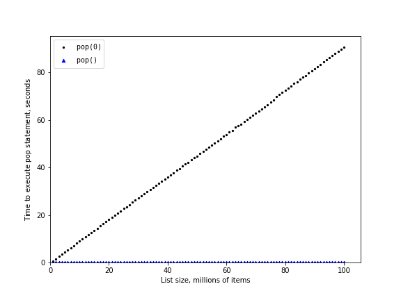
You can see that as the vector gets larger, the time required for erase(v.begin()) also increases, while the time for pop_back() remains nearly constant. This is exactly what we would expect from an $O(n)$ operation and an $O(1)$ operation, respectively.

2.8 Hash Tables (unordered_map)

The second major C++ associative structure is the hash table, unordered_map. As you probably recall, hash tables differ from vectors in that you can access items by a key rather than a position. Later in this course you will see that there are many ways to implement a hash table!

The thing that is most important to notice right now is that the get item and set item operations on a unordered_map are $O(1)$. Another important unordered_map operation is the contains operation. Checking to see whether a key is in the unordered_map or not is also $O(1)$. The efficiency of all unordered_map operations is summarized in Table below:

Operation	C++ unordered_map	Big O Efficiency (average)
copy	unordered_map<int, int> m2 = m1	$O(n)$
access / insert	m[key]	$O(1)$
access existing item	m.at(key)	$O(1)$
insert	m.insert({key, value})	$O(1)$
erase by key	m.erase(key)	$O(1)$
contains	m.count(key)	$O(1)$
search	m.find(key)	$O(1)$
iteration	for (auto& p : m)	$O(n)$
clear	m.clear()	$O(n)$

One important side note on unordered_map performance is that the efficiencies we provide in the table are for average-case performance or amortized analysis. In some rare cases the contains, get item, and set item operations can degenerate into $O(n)$ performance, you can refer to Chapter 6 for more information.

#include <unordered_map>
#include "pythonds3/cppds/dstimer.hpp"
using namespace std;   // iostream/vector/algorithm preloaded by the kernel
int main() {
    cout << setw(10) << "n" << setw(12) << "vector" << setw(12) << "hash" << endl;
    for (int n : {100'000, 200'000, 400'000, 800'000}) {
        vector<int> v(n);
        unordered_map<int, int> m;
        for (int i = 0; i < n; i++) { v[i] = i; m[i] = 0; }
        int target = rand() % (2 * n), hits = 0;
        
        DSTimer t1;
        for (int r = 0; r < 100; r++)
            hits += (find(v.begin(), v.end(), target) != v.end());
        double tv = t1.millis();
        DSTimer t2;
        for (int r = 0; r < 100; r++)
            hits += (m.find(target) != m.end());
        cout << setw(10) << n << fixed << setprecision(3)
             << setw(12) << tv << setw(12) << t2.millis() << endl;}
}

         n      vector        hash
    100000       0.017       0.094
    200000       6.251       0.023
    400000       2.302       0.028
    800000       9.039       0.035

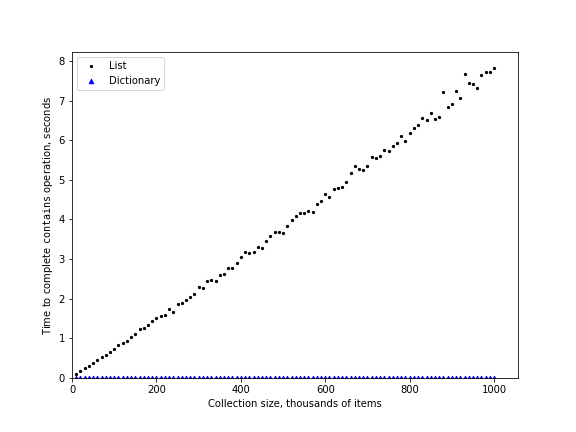
Both containers search for the same target 100 times at each size. The target may be absent, and its position changes between sizes, so the measured vector times need not increase monotonically. std::find uses at most n comparisons; unordered_map::find has average-case O(1) and worst-case O(n) complexity. The figure shows seven fresh measurements with GCC and -O0; timings and random targets depend on the platform, so they need not match the saved notebook output.

display_quiz(path+"dict1.json", max_width=800)

display_quiz(path+"dict2.json", max_width=800)

Exercise: Devise an experiment to verify that accessing an element of a vector using the index operator [] takes $O(1)$ time.

Hint: Measure the time required to access elements in vectors of different sizes and observe whether the access time remains approximately constant as $n$ increases.

// Your code here

from jupytercards import display_flashcards
fpath = "https://raw.githubusercontent.com/phonchi/nsysu-math208/refs/heads/main/extra/flashcards/"
display_flashcards(fpath + 'ch2.json')

References

1. Textbook: Problem Solving with Algorithms and Data Structures using C++ (cppds), Chapter 2 — https://runestone.academy/ns/books/published/cppds/index.html